VI. Einstein’s Theory of General Relativity: History and Mathematics

A Basic Introduction to the Gravitational Field Equation

One learns in elementary physics that g represents the acceleration of gravity having units of distance/(time)² and that E represents the electric field having units of Newtons/Coulomb.

We may not have appreciated when first encountering these two important vectors that the mathematical fields associated with them take identical forms, and that they could be a starting point for understanding Einstein’s general theory of relativity … to come later in this essay.

Elementary physics students encounter gravity in the context of acceleration–the increasing velocity of, for example, an apple falling from a tree. To describe the acceleration of a falling apple, Isaac Newton invented new mathematics – that of differential calculus. Integral calculus, the mathematical flip side of differential calculus, was being developed simultaneously in Germany by the mathematician, Leibniz.

As mentioned, the gravitational acceleration vector, g, and the electric field vector, E, follow identical mathematics. Also, the forces associated with gravity and electrostatics have similar descriptions, and their vector fields are similar, though these similarities are not usually emphasized in elementary courses.

Many will, perhaps, remember their first acquaintance with gravitational acceleration in problems related to calculating the paths of falling bodies such as cannon projectiles or other objects falling to Earth. At the surface of Earth, the gravitational vector has a value of ~9.8 meters/(second)² and pointing toward the center of earth. As the gravitational acceleration vector, g, depends on the distance from earth’s center, this value of ~9.8 meters/(second)² only applies to locations near sea level.

When multiplying the acceleration of gravity, g, with the mass of a test particle, m₀ , one calculates the gravitational force

F = m₀ ‧ g                     (1)

(Force equals mass times acceleration)

When one multiplies the electrostatic field strength by the charge, q_e, one calculates the electrostatic force

F = q_e ‧ E                      (2)

(Force equals the electric field times charge)

Maxwell’s famous equation I of four may be represented as

∇‧E = ρ_e/ϵ₀    ,                 (3)

where ρ_e is the charge density and ϵ₀ is the permittivity of space; see https://ronaldabercrombie.blog/2023/12/17/i-maxwells-equations/,

Though not usually presented in this way, the equivalent equation for g of classical mechanics is

∇‧ g = – 4πGρ_m            (4)

where ρ_m is the mass density and G is the universal constant of gravity.

An often-repeated anecdote is that Einstein on being introduced to an audience before a lecture on his theory of gravitation, was described as “standing on the shoulders of Isaac Newton”, the British father of classical mechanics. He corrected the speaker that it was Maxwell, the Scottish father of electrodynamics who had been more instrumental in guiding his thoughts. These thoughts ultimately resulted in his greatest achievement, the gravitational field equation and are part of the reason he has achieved icon status in physics.

It took him a long time to derive his field equation, but he likely would have pondered equation (4) in the ten-year period during which he worked toward this goal and his general relativity paper of 1916.

A key in the process was his absolute certainty of the equivalence of gravity and acceleration; Einstein once claimed this to have been the “happiest thought of his life”.

Physicists since the time of Galileo and Newton had recognized the importance of velocity and acceleration for describing the effects of gravity on falling bodies. Analysis of gravitational movements using velocity and acceleration requires knowledge of an object’s position and of time. Position and time are silently embedded within the expressions ∇‧ g and ρ_m of equation (4).

After the late 1800s and especially after 1905 when Einstein’s first papers appeared, it became clear that knowledge of the observed position and observed time were much more complicated than had been previously recognized.

If objects move relative to one another, their local time and positions differ, and this difference must be correctly reflected in the math of gravitation. The use of time and position must be adjusted to accommodate relative movements. This concept is at the center of all relativity theory, both Einstein’s special and his general theories.

It wasn’t difficult for Einstein to accommodate such adjustments for the case of steady relative movements between objects (special relativity). Others, Lorentz and Poincaré, had previously done this. However, gravity and acceleration (general relativity) were much more difficult problems to tackle. Einstein spent ten years pondering this, during which time he consulted many luminaries. The answer was to be found in tensor geometry.

That tensor geometry would be useful in the solution was suggested to Einstein by his good college friend, classmate, and student at the ETH, Marcel Grossman. Tensor geometry would allow reference frames existing in different portions of space and time with different movements to harmoniously co-exist. And these reference frames must co-exist even though each remains in a state of constant flux; in other words, each portion of space-time must be perpetually changing, yet it must be seamlessly linked to all others…not an easy problem to solve.

The resulting complications of time, space, location and the geometry of the universe were ultimately addressed in his theory of general relativity. With this, he brought into sharper focus our understanding of the universe.

Space, time, direction, location, and the geometry of the universe

The term, acceleration, means that velocity is constantly changing; Einstein’s happiest thought, as previously mentioned, was that gravity is fully equivalent to acceleration. Therefore, gravity and gravity’s acceleration require that the reference frames of general relativity must be continuously refined and recalculated.

His understanding has been the deepest yet and the most intellectually satisfying (to physicists) description of gravity.

The cosmological constant, Λ, is necessary only for descriptions of very large spaces containing many galaxies^(ref1).  This sometimes-problematic term, when included, may be adjusted to match the expansion or contraction of the universe. It may be ignored for a single galaxy, in which case the field equation simplifies to

G_μν = {(R_μν – ½R 𝑔_μν) = 8𝜋GT_μν/C ⁴} = 8𝜋T_μν                        (1)        

The term on the far-right side of Einstein’s equation (1) is given in geometrized units where C = G = 1, described later.  The symbols containing subscripts G_μν,  R_μν, 𝑔_μν, and T_μν represent tensors of rank two. 

In this essay about general relativity there will be discussions about tensors, one of the essential mathematical tools required to describe this theory.

Tensors come in various ranks, each with a specific role:

• Rank zero tensors: Also known as scalars, these are quantities that have magnitude but no direction.
• Rank one tensors: These are vectors, which possess both magnitude and direction.
• Rank two tensors: Tensors of this rank appear in Einstein’s equation (1) and are crucial for expressing the relationship between spacetime curvature and energy-momentum.

The use of tensors in general relativity is vital because they allow for meaningful comparisons among changing reference frames and for formulating the laws of physics in a way that is independent of the state of relative motion, acceleration, or position.

The left side of the equality in (1) is the Einstein tensor, G_μν, which is made of three parts seen within the inner parenthesis: the Ricci tensor, R_μν; the Ricci scalar, R (a scalar function of position); and the metric tensor, 𝑔_μν (a tensor necessary for measurement of distances in curved space). The right side of the equality contains the stress-energy tensor, T_μν. This tensor incorporates the conserved quantities of energy and momentum; it may be formed as a cross product of two 4-vectors ^{(refs 1,2)}. The tensors of (1), G_μν, R_μν, 𝑔_μν, and T_μν , will be described in more detail. 

Before Einstein’s theory of relativity, classical Newtonian physics in Table II below was thought to be sufficient for the universal description of gravity.

Background.

Newtonian physics. Equations in Table II are useful before tackling general relativity.

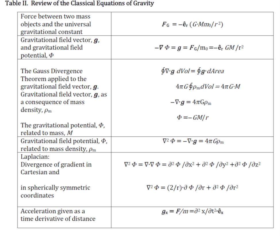
The symbols 𝜌_m, G , 𝒈, 𝜕, d, ∇, 𝜵∙, ∇², M, m₀, r, F , 𝛷, ê_x, ê_r , among others are defined in Appendix I. Vectors are in bold print.   

Special relativity is required background for general relativity. Relativity (special or general) requires extending a local description of time and comparing time and space between moving objects. Both special and general relativity use inertial reference frames in this task.  Inertial reference frames are small portions of space-time, gently floating as imaginary laboratories within which there is no acceleration or gravity. The coordinates of time and space within an inertial frame under observation (x′, y′, z′, and t′) may be compared to an observer’s inertial frame having the coordinate representation (x, y, z, and t). The Lorentzian transformations ( https://ronaldabercrombie.blog/2023/12/17/ii-angles-and-their-role-in-special-relativity/ ) of special relativity below^{(ref 2)} make the comparison between these steadily moving frames in flat space explicit ^{(ref 3)}.

x = γ ∙ x′ + β ∙ γ ∙ t′             (2)

t = β ∙ γ ∙ x′ γ ∙ t′             (3)                   

y = y′ and z = z′ for the case of two reference frames having an orientation such that the steady relative movement is in the x direction only.

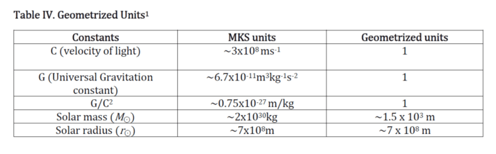
In equations (2) and (3), β = V/C    and γ = 1/(1 – β²)^½, V  is the velocity of the primed (observed) reference frame relative to the unprimed (observer) frame (or vice versa), and C  is the speed of light. In geometrized units, both distance and time are represented as a fraction of the speed of light. Thus, light years, light milliseconds, etc., refer to distances as well as time.

The student may wish to show the invariance of x² + y² + z² – t²  ≡  x′² + y′² + z′²  –  t′²  . (Hint: take velocity to be only in the x direction. Then use equations (2) and (3) to show this expression to be valid in any reference frame.  Also, explain how y = y′ and z = z′ if movement is only in the x direction.)

Components of General Relativity.

The Ricci tensor. Einstein’s great insight was that gravity is equivalent to acceleration. The classical equation for gravity, ∇² 𝛷  =  4πGρ_M, of Table II, which is approximately accurate in small, inertial local frames, may have been a starting point for incorporating his insight about gravity into the new theory.  However, he needed a way to accommodate accelerating, and therefore constantly changing, reference frames.  His friend, Marcel Grossmann, a fellow student at ETH and later a professor of mathematics there, introduced Einstein to tensors and taught him how these may be useful for accommodating the comparison among evolving reference frames ^{(refs 4,5)}.

Understanding tensors in depth would require graduate-level knowledge in this specialized topic, so this essay must use only a few basics.  Einstein’s first attempts settled on the Ricci tensor as a plausible substitute for the Laplacian, ∇ ² of Table II. Like the Laplacian, the Ricci tensor involves derivatives, but it is more complicated because the observed reference frames of general relativity must constantly be re-defined and calculations redone because of acceleration, i.e., because of the changing “gravitational virtual velocity of observed reference frames”, which is the essence and core of gravitation according to Einstein.

Why did Einstein need this accommodation and how did he accomplish his task required for formalizing general relativity? In special relativity, as β = V/C remains constant, the reference frames need be defined only once.  However, in general relativity, the gravitational virtual velocity, V, changes. His theory, which incorporates frame “acceleration,” must accommodate the changing “velocity” and therefore the changing descriptions of reference frames.  We’ll use two frames, one, X, for the observer, and one, Y, for the observed event.  One of these two frames, X or Y, must be continuously redefined, as it would be seen by the other as constantly altering its coordinate framework. The situation has been described as involving “momentary co-moving reference frames” (MCRF)^{(ref 6)}, the meaning of which is that there is a “momentary” but changing difference in “velocity” β between the two reference frames.  Because it is constantly changing, a MCRF represents only a “frozen” view. If the ” virtual velocity” β between the frames were constant, as for special relativity, then this “frozen” view need be defined only once.  General relativity requires that, throughout space-time, reference frames must be repeatedly redefined and compared.

In short, the two compared frames will be designated as “observer” and “observed.”  The “observer” frame is placed at “our location” in space-time; the “observed” frame ultimately takes the space-time position of an event under examination. The intervening space and that of the observed frame must change their descriptions continuously because of gravitational forces.

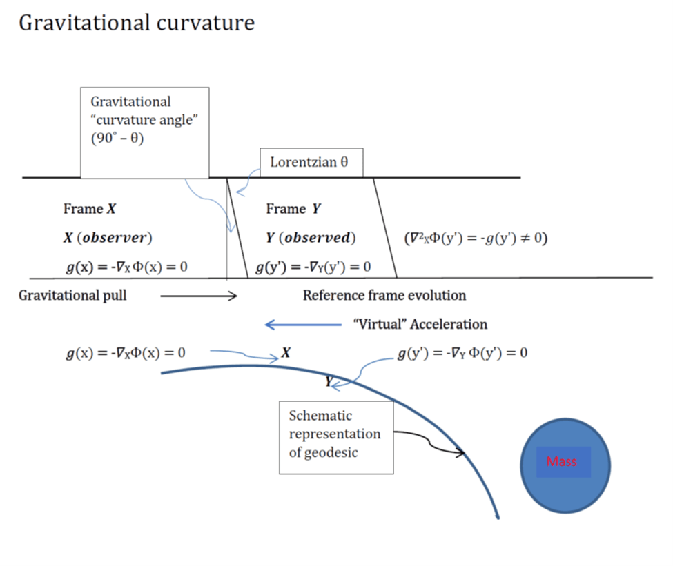
Fig. 1.  A simplified illustration of gravitational acceleration using two reference frames: X , positioned closer to the observer and Y, closer to the observed event.  𝛷 (x) is the gravitational field potential measured from the observer  frame, and 𝛷(y) is this gravitational field potential as measured within an observed frame.  (In the figure a prime is included for the observed frame, Y.) Acceleration within an inertial reference frame is zero according to the definition of an inertial reference frame. However, 𝛻_X 𝛷 (y’) = –𝑔(y’), and 𝛻²_X(y’) do not equal zero because of curvature along the space-time geodesic. Since the two coordinate representations must be placed on compatible terms for the differentiation operation to be meaningful, a coordinate transformation is required. This brings into the calculation the connection coefficients or Christoffel terms. A larger connection coefficient signifies greater curvature. Christoffel (1828-1900) is remembered as the mathematician who expanded the tensor mathematical tools of his predecessor, Bernhard Riemann (1826-1866) with terms that have been given his name.

Appendices II and III are more extended descriptions of the Ricci tensor.  

The Metric tensor. The metric tensor may help clarify the term geodesic. Mercifully, some questions in general relativity may be answered using the metric tensor alone. The metric tensor is given the symbol 𝑔_mn.  Note: this is not the gravitational acceleration vector, 𝑔, even though it is symbolized by the same letter of the alphabet.  Gravitational acceleration, when used as a vector, will be shown in bold print and usually without subscripts.  The metric tensor, 𝑔_mn, defines a mathematical operation for determining the shortest distance, the geodesic, between two points on a curved surface or, in general relativity, two events in curved space-time. It represents a generalized Pythagorean-like calculation for curved relativistic space. The geodesic, the shortest distance between events, must be the same regardless of the reference frame in which it is described. Thus, it must be unchanged by the frame designation of observer versus observed.  An important constraint in relativity theory is that no reference frame should have special place; therefore, the metric tensor must be an invariant tensor.

The square of the infinitesimal geodesic, ds², will be defined using two immediately adjacent reference frames, X and Y, and the metric tensor, 𝑔_mn.  For frame Y (observed) in equation (4), the four incremental vector components are symbolized by dy^q (or dy^r).  In frame X (observer), these vector components are symbolized by dx^m (or dxⁿ).  Each of the indices, m, n, q, and r, take integer values, 0→3, which are the four dimensions (the four co-ordinates) of space-time.

Using the Pythagorean analogy, the square of the infinitesimal geodesic, a tiny displacement along a space-time geodesic curve, is  

ds² = 𝛿_mn{(dx^m/dy^q)∙(dxⁿ/dy^r)}dy^qdy^r  .    (4)

Equation (4) uses the Einstein convention in which if indices appear twice (q and r, m and n), then summations over these indices are implied. This defines the metric tensor, 𝑔_mn, which is an important tensor in relativity theory, as

𝑔_mn = 𝛿_mn {(dx^m/dy^q)∙(dxⁿ/dy^r)}  .     (5)

The metric tensor is a generalized Pythagorean recipe for multi-dimensional curved space-time.  The symbol δ_mn represents the relativistic Kronecker delta, which will be defined shortly.  As written, the metric tensor would be for events in frame Y (observed).  The metric tensor may also be a reverse tensor, 𝑔^mn in which case the roles of the x and y coordinates, i.e., the coordinates of reference frames, X and Y, are exchanged ^{(refs 1,2)}. This is equivalent to switching the positions of “observer” and “observed.”  (The metric, ds, must be invariant if the two reference frames Y and X are interchanged.) 

The standard Kronecker delta, δ_mn, has the value 1 if m = n or 0 if m ≠ n.  Importantly, for the time slot of general relativity, δ₀₀ = -1. Using equation (4) and Einstein’s convention,

ds ² = {-(dx⁰)²/dy^qdy^r+(dx¹)²/dy^qdy^r+(dx²)²/dy^qdy^r+(dx³)²/dy^qdy^r}dy^qdy^r  .   (6)

In “flat” Lorentz-Minkowski space, ds² = – (dx⁰)² + (dx¹)² + (dx² )² + (dx³)² = – (dy⁰)² + (dy¹)² + (dy²)² +(dy³)².   In the more familiar notation of special relativity, ds²= –dt² + dx² + dy² + dz² =   –dt′² + dx′² + dy′² + dz′².  The physics student should verify this equality by evaluating equation (6) and following procedures like those of previous student exercises. 

To recap, operation of the metric tensor generates a scalar, which is a measure of the space-time separation between two events in 4-D space-time.  The accumulated sum of ds increments, i.e., the space-time separation or “world-line” between events must have the same value; that is, it must be invariant of the reference frame in which it is calculated.  But it will of course change with the event being observed. Repeating, the infinitesimals ds when summed along the geodesic form an invariant world line (the space-time separation) as represented in the schematic of Figure 1. 

In special relativity (a. and b.), and in the curved space of general relativity (c. and d.), the metric, ds, may take several forms.  Some are shown in Table III.

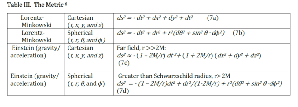
Equation (7d.) results from evaluating equation (6) using spherical coordinates^(refs1,6,7).

All Equations of Table III are given in geometrized units with C = G = 1. 

Engineers, who have been tasked with precisely controlling communication satellites must know that the gravitational acceleration vector, 𝑔, acting on these satellites is governed by ^{(refs 6,1)}

𝑔 = GM∙ ê_r/r²(1-2GM/C²r) = M∙ ê_r/r²[1-2M/r] ,   (8) [C = G = 1]

rather than 𝒈 = GM∙ ê_r /r²  as was represented in Table II.  Without this correction, the satellite communication system between earth and orbiting space satellites would not function properly.

The Ricci scalar.  Tensor mathematicians have procedures for contracting a tensor R_μν  to a scalar; R = R^μν𝑔_μν  =  𝑔^μνR_μν  .  This involves an inner product of R_μν with the metric tensor, which eliminates terms in which μ ≠ ν.  The Ricci scalar, a compact measure of local space-time curvature^(ref1) was introduced into general relativity theory by the mathematician David Hilbert, as described below.

The Ricci tensor is not a sufficient substitute for ∇ ² of Table II.

Einstein needed to equate the two sides of his field equation.  For tensor equations, this requirement is complicated.  As mathematicians were to inform Einstein, the covariant divergence of the Ricci tensor alone does not equal zero (that is, ∇ ∙ R_μν ≠ 0).  Einstein’s first trial for the left side of his field equation had been using the Ricci tensor alone.  However, he realized that he had to consider that the covariant divergence of his energy-momentum tensor on the right side of this equation was zero. So, he had a problem ^{(ref 4)} if this equation was to represent a general description of gravity and space as he had wished.  He needed help from world-class mathematicians, and he likely received some from renowned German mathematician David Hilbert.  Hilbert submitted a paper on this topic in the fall of 1915 ^{(ref 8)}, but this followed a summer visit from Einstein during which they discussed the subject.  Hilbert never claimed any credit for the solution to the covariance problem, though his singularly authored paper on this subject included an explicit solution, an event that led to bad feelings between the two men ^{(ref 4)}. 

Einstein finally settled on a version of his equation that was general and valid in any reference frame or coordinate system as is shown in equation (1); the covariant divergence (𝛻 ∙) of both sides of this equation was zero, which was deeply satisfying to Einstein as to the mathematicians.

𝛻 ∙ (R_μν – ½R𝑔_μν) = 0 = 𝛻 ∙ (8𝜋T_μν),                         (9)

Where 𝑔_μν is the metric tensor.  It may be important to point out that

𝛻 ∙ 𝑔_μν = 0                                           (10)

in any reference frame.

However, 𝛻 ∙ R_μν ≠ 0, but rather 𝛻 ∙ (R_μν + ½R 𝑔_μν) = 0, a detail that Hilbert helped to resolve.

To summarize, after some initial trials that proved only partially fruitful, Einstein incorporated the Ricci tensor minus the term (½R 𝑔_μν), which made the covariant divergence of the left side of his field equation equal to zero and equal to the covariant divergence of the stress energy tensor on the right side. The stress energy tensor contains the conserved quantities of relativistic mass-energy and momentum^{(ref 1)}.  His result (equation 1) was presented in a paper submitted by Einstein in the fall of 1915 ^{(ref 9)}.  In geometrized units where C = G = 1, the field equation could now be written in a compact form. The important addition of the term, – ½R𝑔_μν completed Einstein’s ten-year quest.

Schwarzschild radius. The radius of our sun, r_⊙ is much larger than its mass, M_⊙ (in geometrized units).  Therefore, any general relativity correction term for gravitational attraction (equation 8 or Table III.) at the sun’s surface would be small, though not zero.  However, for stars that collapse to a radius equal to twice their mass (in geometrized units), an apparent “singularity” exists at r = 2M^{(ref 7)}.  To a distant observer, gravitational acceleration, 𝑔, would appear infinite at the Schwarzschild radius of r = 2M; also, time would appear to stop there. 

Student practice with units: If our sun were to become a black hole, its mass would be compressed into a sphere with a radius of only three kilometers. Conclusion: A black hole represents a very dense object.

Student exercise:
“Why is space-time curved, and why do space and time seem to disappear at the surface of a black hole?” 

A space-time “angle” of special relativity, θ, (in the Figure), as viewed from an observational or “stationary” frame, may be described using an application of Lorentz’s transforms.

sin θ = τ/t = (1 – β²) ^½      (11)

According to Einsteins equivalence of gravity and a virtual acceleration, an object may have a virtual gravitational velocity even though it would appear stationary to an observer. Taking the observational frame perspective, equate an observed particle’s kinetic plus its potential energies to zero, assuming this to be its value at hypothetical infinity in a region of flat space-time. This procedure may be repeated in a second stationary position using conservation of energy and a comparison of the two “momentarily stationary (MCRF)⁶” and conceptually interchangeable frames, one at infinity and one at location r : 

0 = P.E./m + K.E./m = –G∙M/r + ½V ²  (with C=G=1)

β² = (V/C )² = 2GM/rC ² = 2M/r   .   (12)

With this substitution:

θ = arc sin√(1 – 2G∙M/rC ²) = arc sin√(1 – 2M/r)    (13)

in geometrized units. 

At r = ∞, which is the hypothetical position of the reference point, no space-time curvature exists.  How does curvature change as the observed location drifts toward a mass, M?  Equation (13) and the Figure represent a Lorentzian angle, θ, and its complement, the gravitational curvature angle (90° – θ) as shown in the Figure.  

As there is no curvature at r = ∞, the “curvature angle” =  90° – θ = 90° – 90° = 0°: there is no gravitational curvature in the region of flat space-time. Curvature begins as an object is imagined drifting from infinity (as r decreases).  At the Schwarzschild radius, r_S  = 2M  and θ = 0° . At this location, time for the observed object appears to stand still and the gravitational “curvature angle” (90° – θ) appears to take its maximum value of a 90° angle. For the distant observer, the surface defined by the Schwarzschild radius seems a strangely unique and forbidden horizon.

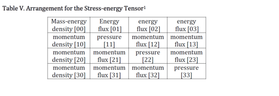
Final component of General Relativity: The Stress-energy tensor. The stress-energy tensor, T_μν, of Einstein’s gravitational equation has interpretations shown in Table V. In this simplified description, the mass elements of this tensor will be imagined as a collection of cosmic “dust particles”, which are described from within the rest frame of the particles.  However, wherever gravity exists, there is virtual acceleration. As acceleration is involved, there must be a changing virtual velocity for these particles. The description of particle movement must be represented in the stress-energy tensor from an observer’s perspective. 

This stress-energy tensor has several requirements. It should be symmetrical (as G_μν is symmetrical); it should have zero covariant divergence ^{(ref 8)}, and 8𝜋GT_μν/C⁴ should reduce to 4𝜋G𝜌_M in the classical limit. As previously stated, this tensor includes the mass of dust particles as measured within the observed reference frame, Y, but their “virtual gravitational velocities” as seen from the perspective of the observer’s frame.

Using as a guide the requirement that m² + p² = E², from special relativity, the stress-energy tensor, T_μν,may be viewed as a composite of two mass/energy- momentum 4-vectors as described below.

One mass/energy-momentum 4-vector for an “event” within frame Y as seen from the observer frame may be written as:

U_μ^X = m ∙ γ(1ê_t^X + β_xê_x^X + β_yê_y^X + β_zê_z^X)/Vol                   (14)

Where ê^X_μ  are the unit basis vectors of the observer’s frame.  The symbol m represents the mass of the particles in the observed frame, and the expression Vol represents the (3-D) volume elements for particles (in the observed frame, Y).  Here, the subscript μ takes values of (0=time), (1=x), (2=y), (3=z). The symbols γ and β have their meanings from special relativity. The symbol β represents the virtual, gravitational, velocity of the two frames. Acceleration between frames being equivalent to gravitation following Einstein’s description. 

A second and similar vector may be defined as

Ū_ν^X = n₀ ∙ γ(1ê_t^X+ β_xê_x^X + β_yê_y^X + β_zê_z^X)               ,               (15)

where n₀ is the particle count within the volume, Vol , of the observed frame Y .

These two vectors generate the 4×4 stress-energy tensor of rank two:

T_μν = (U_μ ⊗ Ū_ν)   .     (16)

The subscripts μ and ν are the four components:  resting mass energy (0) for the time position, and (1, 2, and 3) for the three orthogonal components of momentum, p_x, p_y, p_z,.     

Constructing a tensor as the cross product of two similar vectors (in Table V) has the effect that a) energy flux [01] = momentum density [10]; b) momentum flux [12] = momentum flux [21], etc., and c) satisfies that this tensor is symmetrical.

The upper left-hand corner term [00] is representative of mass/energy density mn₀  γ²/Vol or 𝜌 ∙γ² within the observed frame as would be seen by the observer.  The other terms along this row represent mass/energy density multiplied by a velocity term. The (t, x) or [01] position is said to represent “mass/energy flux” (mn₀ β_x γ²/Vol) or 𝜌β_x γ², which is the same as the (x, t) term in the [10] position. This term is given the name “momentum density”.  Also, “momentum flux” [12] (mn₀ β_xβ_y γ²/Vol) or 𝜌β_xβ_y γ²) is the same as “momentum flux” [21].  The diagonal terms have units of kinetic energy divided by volume, which are units of pressure ^{(refs 1,6)}.  Einstein’s insight in devising this tensor description of mass/energy and momentum for his field equation seems both complex and inspired to most of us, reinforcing our appreciation of his deep insights and the undeniable genius of his thinking.

General relativity predictions (two successes)

The bending of light around a massive object: Einstein calculated the acceleration of a photon as it travels near the sun.  An incorrect qualitative prediction had been suggested earlier by others long before Einstein’s general relativity theory appeared.  Einstein’s correct calculation ^{(refs 10)} (even before his final version of the field equation had been completed) yielded a value for the deviation of light’s path as twice that of earlier calculations.  His prediction was made well before light bending was measured in 1919.

Light bending was observed during a scientific expedition to photograph a distant star, which could be seen just beyond the edge of the sun as the sun appeared to pass across the sky.  This arrangement for photography of the star was possible only during a solar eclipse because the sun’s bright light would have otherwise overwhelmed that of the distant star.  The famous expedition was led by a group of English physicists, including Arthur Stanley Eddington and Frank Watson Dyson.  Their observations seemed to confirm Einstein’s calculation.  Subsequent measurements have done so reliably ^{(ref 4)}.

Perihelion of Mercury: According to Kepler and Newton, any planet (Mercury for example) will remain in a stable elliptical orbit around the more massive sun if there are no forces other than the central attraction of the sun’s gravity.  However, the other planets, which also have an elliptical orbit and move in the same direction and roughly the same orbital plane as Mercury, exert a gravitational pull.  As for Mercury, which is the closest planet to the sun, this perturbation of the other planets causes its orbit to be unstable.  Mercury’s major axis rotates a small amount with each full transit around the sun.  A classical Newtonian calculation for the pull of the other planets predicts that the perihelion of Mercury’s ellipse should rotate by 532 arc seconds each Earth century ^{(ref 11)}. This is smaller by a significant amount than astronomical observations.  As Mercury is closest to the sun, Einstein reasoned that a general relativity correction for the sun’s gravitational acceleration should be significant.  Although G is constant, gravitational acceleration, 𝑔, is not constant and changes with the planet’s distance from the sun (equations 8 and 18).  Using a similar methodology to that of his calculations concerning the bending of light’s path by the sun’s gravitational pull (before his final version of the gravitational field equation had been completed), Einstein was able to calculate the correct perihelion shift.  This added 43 arc seconds per Earth century to the adjustment of Mercury’s orbit, and it fit with the astronomical observation of 574”  ≃  532” + 43” per century.

These early successes led to rapid acceptance of the general theory of relativity, which has now become an integral part of the modern understanding of the universe.

Black holes: These strange objects of our universe have achieved special status in our imagination.  Princeton physicist John Wheeler gave them the name “black holes” ^{(ref 1)}.  One could make a simple (and incorrect) classical estimate of the radius of a black hole as follows:  In Newtonian physics, the amount of gravitational acceleration required to maintain an object in a circular orbit at a radius, r , and with a velocity, V, is

𝑔 = V ²/r .      (17)

The Newtonian value of gravitational acceleration at a distance r from an object of mass, M is

𝑔 = GM/r ²= M/r ² (In geometrized units where G = 1).      (18)

Equating these expressions for 𝑔 and substituting the velocity of light, C, for the speed, V, of the orbiting entity provides a classical estimate for the radius of a light path around the attraction center of a concentrated mass M as

r = GM/C ² = M  (In geometrized units where G =C=1).    (19)

The fact that photons are without mass is not relevant in general relativity as curved space determines the photon’s path. 

From equations (7d), (8), or (13), we know that the correct relativistic Schwarzschild radius, r_S, is twice this value or

r_S = 2M.                               (20)

A factor of two is needed in this case, as well as the earlier solar eclipse calculation, to make the classical estimates compatible with general relativity theory.

Closing remark. Einstein was clearly a genius. Along with Newton, Maxwell, and a few others, he is considered among the most influential physicists of all time.  But he did not work alone.  He was a brilliant collaborator.  He consulted with friends and undoubtedly with his first wife Mileva Marić (1875-1948) a Serbian-born physicist and mathematician.  Only one woman had finished the full program at ETH before her.  His friends Marcel Grossman and Michele Besso were key collaborators as well.  Einstein was surely the creative and intellectual leader, though we must believe that others made important contributions and necessary critiques at critical times.  We should also consider that Einstein lived in an era of many great and influential scientists whom he consulted or whose works he read. These include Lorentz, Poincaré, Minkowski, Hilbert, and Plank. All these living greats of Einstein’s time were preceded by Riemann, Christoffel, Newton, Maxwell, and Galileo, among others. 

It may be relevant to point out that Einstein’s first attempts were not always complete. There were earlier iterations of his field equation of general relativity before he published its final form in 1916.  So, one needn’t always be perfect on the first try to be remembered in science (perhaps a poignant lesson for students). Einstein, in addition to his vast intellect, had another characteristic which propelled him to greatness: he was able to think independently and very deeply. “Thinking outside the box” (if we may take the liberty to substitute “thinking outside the local inertial reference frame”) was his natural practice before this became a familiar phrase.

Appendix I: Definition of symbols

𝜌_M          Mass density

G            Universal constant of gravitation

C            Universal speed of light

𝑔            Gravitational acceleration vector

d or 𝜕       Derivative or partial derivative

𝛻              Gradient, a partial derivative in all directions

𝛻∙             Divergence, derivative of each component of a vector

𝛻²            Laplacian, divergence of gradient

M             Mass of larger body

r               Distance between mass centers

F              Gravitational attraction force vector

m₀           Test mass

E              Energy

p             Momentum vector

V              Velocity between inertial reference frames

𝛷              Gravitational field potential

ê_x , ê_r       Basis vectors (orthogonal unit vectors)

θ              The Lorentzian angle in special relativity

“angle” = 90 ̊ – θ     The distortion, or gravitation angle, of an observed reference frame

giving rise to space-time curvature in general relativity

Appendix II: Ricci tensor

The Lorentzian transformations of equations (2) and (3) are given compact expressions in equation (1A).  Though equation (1A) may appear different from equations (2) and (3), it is the same.  Vector A having coordinates A_r^Y may be “transformed” from reference frame Y (observed) to reference frame X (observer), that is, the vector coordinates in frame Y may be re-expressed using the coordinates of the reference frame X. The lower-case, x and y, will designate the four coordinates of the vector A in the two inertial reference frames, designated as X and Y.

A_m^X = (dx ^r/dy ^m)A_r^Y                      (1A)

A_r^Y are the four scalar coordinates of a vector in frame Y. As first introduced in Table II, ê_r^Y are the basis vectors or unit eigenvectors of frame Y.  Each coordinate basis vector, ê_r^Y, and each scalar component of this vector A_r^Y, in frame Y also has a representation in the other frame, X. 

In the Einstein convention, if an index appears twice in one term, then a summation is implied.  For example, (dx ^r/dy ^m) A_r^Y  in equation (1A) implies summation over all integer values of the indices, r = 0, 1, 2, 3. This   must be repeated for each value of m.   A student exercise, below, may help clarify. 

Student exercise:  Show that equation (1A) is equivalent to equations (2) and (3).

Answer: Substitute A₁^Y =x ′  and A ₀^Y=t ′ ; A₁^X=x   and A₀^X= t  ; x⁰ = t ; x¹ =x ; y⁰ = t’; y¹ = x’; dx ¹/dy ¹ = dx/dx′ = γ, dx¹/dy ⁰= dx/dt ′= βγ,  dx ⁰/dy ¹= dt/dx ′ = βγ ,  dx⁰/dy⁰ = dt/dt ′ = γ , to recover the familiar Lorentzian transformations. The student may wish to expand this to include the two other spatial dimensions.

Likewise, if one transforms a “simple” second-order tensor such as T _rs^Y=A_r^Y ⊗B_s^Y,  then the following procedure would be used for cross product of the components of the two vectors A_r^Y and B_s^Y:

T^X_mn = {dx^r ∙dx^s/dy^m ∙dyⁿ} T^Y_rs  .  (2A)

The tensor projections are of the Y coordinates (observed) onto the X frame (observer), leaving no “stone unturned,” so to speak, in choosing all possible combinations.  An example of a tensor that transforms in this way is the metric tensor.

The Ricci tensor, R_μν , though, is a more complicated second-order tensor. The operation of a second derivative ^{(ref 1)} in curved space includes terms that do not appear explicitly in equation (2A) … these are the connection coefficients (or Christoffel symbols).  Upon including these, the Laplacian operation becomes the Ricci tensor:

∇² 𝛷 ⇢ ∇∙𝑔 ⇢ R_μν .          (3A)

How does the Ricci tensor use Christoffel symbols to accommodate changing coordinates in general relativity?  The simple answer is that the connection coefficients of the Ricci tensor bring together the evolving reference frame’s basis vectors, ê, allowing this comparison to become possible. A more involved answer is given in Appendix III.

Appendix III:  Connection coefficients, Christoffel symbols, and the “angle” of curvature 

The connection coefficients are symbolized as, Γ_βγ. One way to define these is by using two adjacent reference frames. The connection coefficients used for accommodation of basis vectors may be represented as

Γ_βγ = ⟨ ê_α^X, 𝛻_γ^X ê_β^Y ⟩  .       (4A)

The abbreviation 〈 , 〉 indicates a comparison between entities separated by the comma (that is, a mathematical projection of one upon the other).  Each reference frame has a set of unit basis vectors: for Y (observed), these are ê_β^Y; for  X , (observer) these are ê_α^X .  The full covariant differentiation of the acceleration vector, 𝑔, in Y requires differentiation of the scalar components of this vector (as in equation 2A) but also it must include “differentiation” of the unit basis vectors as represented in (4A). Differentiation of the scalar components, A_r^Y, has already been included in the standard transformations shown in equation (2A). For differentiation of the unit basis vectors (4A), ê_β^Y, of 𝑔 in frame Y, one must use the coordinate system of the adjacent (the observer) frame X:  d( ê_β^Y )/dx_γ.  (Otherwise, the differentiation would yield a value of zero.) Including the connection coefficient term adds “space-time curvature” at the intersection between frames and fulfills the requirement for the second component of the derivative operation. Stated symbolically,

d ê_β^Y /dx_γ = Γ^α_βγ  ê_α^X               (5A) 

Briefly, a full differentiation of the basis vectors for 𝑔 in frame Y requires this factor, Γ_βγ , which is a measure of local space-time curvature.

In a more standard notation ^{(ref 1)}, the connection coefficient may be symbolized as

Γ_βγ = ⟨ω ^α, 𝛻_γ𝒆_β⟩   ;

the first slot in the bracket uses the observer’s basis vectors, the second slot uses the observed frame’s basis vectors.

An important point to emphasize, though, is that Einstein and others ultimately realized that the Ricci tensor in curved space-time, though quite complex with the inclusion of connection coefficients was not a sufficient replacement for the classical Laplacian for his field equation.  A modification had to be made in the form of a subtraction term, ½ R𝑔_μν.  Adding this term produced the final covariant version of the field equation and formed what is now known as the Einstein tensor as presented in equation (1).

Appendix IV:  

Covariant divergence. In the discussion, phrases “covariant divergence” and “covariant derivative” appear.  A covariant derivative is akin to a partial derivative for one dimension.  Covariant divergence includes partial derivatives in multiple dimensions.  The adjective covariance signifies that these operations remain valid following a transformation from one reference frame to another.

Invariance. In any space, including curved space, the covariant derivative and divergence operations should remain valid for any reference frame if it is to satisfy the invariance requirement.  Transformations between adjacent frames under acceleration bring additional terms into the calculation (the Christoffel terms of Appendix III).

The far field approximation refers to values of r  that are much greater than the Schwarzschild radius.  This approximation allows equation (7d) to be expanded as a series in 2M/r giving the equation (7c) ^{(refs 1,6)}.

The stress-energy tensor may be formed as a cross product of two energy-momentum 4-vectors ^{(ref 1)}.  It incorporates the mass, m, of all dust particles of the observed reference frame and a 3-vector,  β_xê_x +β_yê_y+β_zê_z  representing that frame’s gravitational or “momentary virtual velocity”, which is calculated using the observer frame perspective.   Momentum and energy are locally conserved quantities even in relativistic physics; the covariant divergence of the stress-energy tensor is zero ^{(refs 1,4,6)}.

References

¹ Misner, Charles W., Thorn, Kip S., and Wheeler John Archibald, Gravitation, Princeton University Press, 2017

² Taylor, Edwin F., Wheeler, John Archibald, Spacetime Physics, W.K. Freeman, and Company, 1966

³ Two papers on special relativity Albert Einstein: Zur Elektrodynamik bewegter Körper, Annalen der Physik 17, 1905, 891–921; Albert Einstein:  die Trägheit eines Körpers von seinem Energiegehalt abhängig, Annalen der Physik 18, 1905, 639–641, 

⁴ Pais, Abraham, “Subtle is the lord…” The Science and the Life of Albert Einstein, Oxford University Press, 1982

⁵ Einstein, Grossmann, Z. Math. Physick, 1914, 63, 215-225; and Einstein, A. and M. Grossmann, Z. Math. Physick, 1913, 62, 225-261

⁶ Schutz, Berbard F., A First Course in General Relativity, Cambridge University Press, 1985

⁷ Schwarzschild, read by Einstein: “Über das Gravitationsfeld eines Massenpunktes nach der Einsteinschen Theorie”, Sitzungsberichte der Deutschen Akademie der Wissenschaften zu Berlin, Klasse fur Mathematik, Physik, und Technik, 1916, 189. And K. Schwarzschild, “Über das Gravitationsfeld einer Kugel aus inkompressibler Flussigkeit nach der Einsteinschen Theorie”, Sitzungsberichte der Deutschen Akademie der Wissenschaften zu Berlin, Klasse fur Mathematik, Physik, und Technik, 1916, 424.

⁹ Definitive general relativity paper: Albert Einstein: Die Grundlage der allgemeinen Relativitatstheorie, Annalen der Physik 1916, 49

⁸  Hilbert, Gesellschaft der Wissinschaften, Nac.  Ges. Wiss.Goettingen 1916, 395.

¹⁰ Perihelion shift, before his final definitive paper: Einstein, A.  “Erklarung der Perihelbewegung des Merkur aus der allgemeinen Relatvitatstheorie”, Sitzungsberichte der Preussischen Akademie der Wissenschaften zu Berlin,  1915, 799-801

¹¹ Chris Pollock, Mercury’s Perihelion, March 31, 2003, http://www.math.toronto.edu/~colliand/426_03/Papers03/C_Pollock.pdf

Other resources

Walter Isaacson, Einstein, His Life and Universe

(DeGrasse Tyson), Neil, Astrophysics for People in a Hurry

(Lang): Lang, Serge, Linear Algebra, Addison-Wesley, 1967