III. Least Action Principle of Classical Mechanics

A bedrock principle of physics astonishing in its simplicity yet sometimes difficult to apply in realistic situations

Two phrases in the preceding title may require some explanation: “least action” and “classical mechanics.”  The least action principle recalls an observation once heard from a clever fellow student that “nature is fundamentally lazy.”  That is, nature will take the path requiring the least action. The phrase classical mechanics is usually about understanding the movements of objects large enough to be seen. Surely, we have all at times wondered how things move.  At the age of three, Scottish physicist James Clerk Maxwell questioned his relatives as he saw interesting things moving about: “What is the go ‘o that?” he would ask. 

Visible movements

Though all things move, some movements are larger and seem more significant. Celestial bodies were important to many ancient civilizations. They believed that an unknown force propelled these across the sky and supposed that the paths of planets and stars could foretell our future on Earth. This undoubtedly stimulated their curiosity about the night sky and focused their attention on the heavens.

Eventually we gained a deeper understanding of celestial movements.  We can trace our accumulating knowledge in the writings of Galileo, Kepler, Newton, and Einstein, who pondered the skies as they sought answers to that same persistent question, “What is the go ‘o that?”  As ancient peoples thought they might be able to predict our future on Earth through studying the paths taken by planets and stars, scientists focused their attention instead on trying to predict the future of the planets, stars, and galaxies within the unfolding universe.

Classical mechanics concerns movements of all things visible ― including the planets.  It allows us to predict these with great accuracy. To be quantitative, predictions require that a set of parameters be chosen.  Time, position, velocity, as well as mass, force, energy, and momentum could be considered.  So, which of these parameters must one use to make predictions? As mathematicians and physicists soon realized, some flexibility is allowed.  However, the choice made for the parameters of motion often determines how easily these problems may be solved.

One could take, for example, a numerical (or finite-difference) approach.  This method is considerably easier now because of computers.  The starting position, velocity and mass of each particle, the forces acting, and Newton’s laws of motion are sufficient for a numerical solution. However, as one might imagine, it is a tedious procedure to decipher movements using this step-by-step approach. It involves a numerical approximation of Newton’s second law (Force = mass x acceleration), knowledge of all the forces of interaction, the individual masses, and billions of calculations. The approach is similar (roughly speaking) to what modern weather forecasting models do.  As approximation errors accumulate for any numerical procedure, such models will be of value during a short window of time, and for only a limited expanse of space.

By contrast, an analytical approach is not hindered by accumulating errors, nor is it limited in time or expanse of space.  A correct analytical solution remains correct forever.  However, the drawback of the analytical method is that it nearly always involves using a simplifying model: that is some necessary idealizations of the real world are needed to render the analytical approach practical.

Sophisticated methods, such as those of Euler, Lagrange, Hamilton, and Jacobi, are helpful in solving problems of motion. They transform Newton’s second law into path integrals and equations based on the minimum action principle.  The path integral and minimum action procedures will typically reduce the number of parameters required for a solution.  Even so, a complete closed-form (or algebraic) solution is never guaranteed using this method. 

The Least action principle: The path taken by a single particle (or a group of particles) will be that (those) path(s) for which the accumulated differences between the kinetic and potential energies is the minimum.  This principle seems astonishingly simple and leaves some understandably a little awestruck on first hearing of it.  To be more precise, it is an extremum (maximum or minimum) rather than the minimum that is required mathematically.  However, we expect nature not to be wasteful of energy, so the minimum is somehow more satisfactory.

Four examples of movement problems follow. They are given as a prologue for Essays  IV (thermodynamics/statistical physics) https://ronaldabercrombie.blog/2023/12/14/iv-brief-summary-of-thermodynamics-and-statistical-physics/ and V (quantum mechanics) https://ronaldabercrombie.blog/2023/12/15/v-a-conversation-about-quantum-mechanics/, to help develop familiarity with some analytical procedures, and to illustrate limitations of these methods. These examples use the Lagrangian technique, which is based on the least action principle.  For a derivation of the Lagrangian equations of motion, one may consult any classical mechanics textbook.

 Problems in classical mechanics

1. Planetary movement

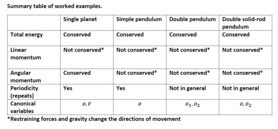
The first example is that of a planet’s movement around its star.  The planet orbits the center of mass of the system. For our solar system, since the sun is much more massive than the Earth, the center of mass of this system is very near the center of the sun.  The other planets and the Earth’s moon must be ignored, which is a simplification necessary to make an analytical solution possible.

The solution uses only two variables: the generalized coordinate, ø , describing the angle of the Earth’s annular motion about the sun, and the parameter, r , describing the distance from the center of the Earth to the system’s center of mass within the sun.

L signifies the Lagrangian; T is the kinetic and V  is the system’s potential energy.  

L = T – V .                           (1)

A first derivative with respect to time may be signified by a single prime (‘ ) over the variable.

The Lagrangian equations of motion using generalized coordinates q_i and q’_i   ^{(ref 5,6)} are

d(𝜕L/𝜕q’_i)/dt – (𝜕L/𝜕q_i) = 0     (2)

where q_i represents position; the parameter for velocity is q’_i . 

A separate Lagrangian equation must be written for each of the coordinates, r and ø.

Writing the system’s kinetic and potential energies in these chosen coordinates, r and ø, the Lagrangian, L , is

L = T – V = ½mr′ ²  + ½m(r ø′ )²   + GMm/r   .     (3)

The symbols M  and m  ^{(footnote 3)} are the mass of the sun and the Earth respectively ^{(footnote 7)}, and G is the universal gravitation constant. From equation (2), the differential Lagrangian equations of motion for ø are

d(𝜕L/𝜕ø′ )/dt – (𝜕L/𝜕ø) = 0  ,     (4a)

and for r

d(𝜕L/𝜕r’ )/dt – (𝜕L/𝜕r) = 0  .    (4b)

From (4a),

 d(mr²ø’ )/dt  = 0.  (5)

Equation (5) states that an entity

mr² ø’ = 𝓛 ,           (6)    

the angular momentum of the Earth in its orbital path about the sun, must not change with time.  This is equivalent to Kepler’s rule of equal areas being swept through space in equal time by the planet’s orbital path and represents conservation of angular momentum for planetary orbits.

The result of equation (6) will become useful in Lagrange’s equation (7), as a substitute for ø‘.

Using the expression (3) for the Lagrangian, L, and applying equation (4b) for the generalized coordinate, r, gives equation (7), where a double prime (” ) represents the double time derivative.

mr′′ –  mr(ø‘)² + GMm/r ²   = 0.   (7)

By substituting ø’ from equation (6), equation (7) becomes

mr′′ – 𝓛²/mr³   + GMm/r²   = 0 .    (8)

(The independent variable of time appears in equation (8) as r′′ = d²r/dt² ). For an analytical solution, two of the variables seen in equation (8), r and t must be replaced:  for r, substitute 1/u, and for Δt , substitute a generalized coordinate of the orbital angle, Δø. This is done as mr² Δø = 𝓛Δt   (equation 6) and rearranging to 1/Δt = 𝓛/( Δø ·mr²).  One then makes the following substitutions:

r = 1/u                  (9)       

𝜕/𝜕t = (𝓛u² /m) 𝜕/𝜕ø   ,       (10)

r′′ = -(𝓛² u² /m² ) 𝜕²u/𝜕ø ²  .    (11)

Equation (11) may not seem obvious; to illustrate this, one may use equation (9) and show that

r′′  = 𝜕 (-u’/u² )/ 𝜕t  .    (12)

Then substitute with equation (10) to change the independent variable from t  to ø, leaving

r′′  =(𝓛u²/m) 𝜕 (-𝓛u² /u²/m[𝜕u/𝜕ø])/𝜕ø .    (13)  

Within the second parenthesis of equation (13), u² in the numerator cancels u² in the denominator; so only constants and the derivative within brackets, [𝜕u/𝜕ø] remain, which leaves equation (11).  This allows differential equation (8) to be re-written:  

𝜕² u(ø) /𝜕ø²  + u(ø) = GMm²/𝓛² = const. = 1/a             (14)

1/a  abbreviates the collections of the constants in GMm²/𝓛².  The solution: u(ø) = f·cos(ø) + 1/a  satisfies equation (14) and includes the constants “f  ” and “a ”. These terms may be rearranged producing  

r = 1/u(ø) = a/(1+ ε cos(ø)) ,     (15)

with

a = 𝓛²/GMm² and ε = f·a       (16)

Depending on the value of ε, equation (16) represents a hyperbola, a parabola, an ellipse, or a circle for the orbiting planet.   A convenient way to visualize this is by using a free online graphics calculator such as GeoGebra. https://www.geogebra.org/classic .The generalized coordinates r and ø, may be converted to Cartesian coordinates, x and y, for use with the calculator.  Equation (15), re-expressed in Cartesian coordinates, is

(x² + y²) ^½ + ε x = a  .   (17)

Values of the constants, a  and ε, need to be specified.  For convenience set a = 1. The plotted equation will be a circle (if ε = 0), an ellipse (if 0 < ε < 1), a parabola (if ε = 1), or a hyperbola (if ε > 1).  This includes all possibilities for planets, pseudo-planets, comets, and asteroids moving within the sun’s gravitational field, and those objects that leave our solar system never to return.

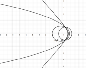
Fig. Orbits about an attraction center located at the origin (x=y=0) and calculated from equation (17). The result is a circle, an ellipse, a parabola, or a hyperbola depending on the value of ε. If the parameter a were 2 rather than 1, the orbital size would double.

2. Simple pendulum and time

By the 17^th century, pendulum timekeeping had come into use.  When everyone comes to an agreement on a common time, many activities of our separated but interacting lives could proceed more efficiently.  The pendulum, which was used by Galileo Galilei in his laboratory and pendulum clocks that were designed by Christiaan Huygens in the 17^th century, could be accurate to a fraction of a second.

The simple pendulum is composed of a large mass, M, with a supporting thin rod of length, r, having negligible mass.  The pendulum mass and the rod length are presumed constants. The angle from the vertical, ø, of the pendulum is the dependent variable, and time, t, is the independent variable.  The distance along a cord from the lowest point of the pendulum’s mass (at the rod’s vertical position) to another position along its arc is given the designation, s. The vertical elevation of the mass M at any point along this arc is represented as Δh .

Using geometry, 

Δh/s = ½s/r,    (18)

and trigonometry,

½s/r = sin (ø/2) .           (19)

Combining equations (18) and (19) gives

Δh = 2r sin² (ø/2) .         (20)

The change in the potential energy, V, of the mass is

V = 𝑔mΔh = 2𝑔mr  sin²(ø/2) .                  (21)      

The full Lagrangian expression is

L = T – V = ½mr² øʹ² – 2𝑔mr sin² (ø/2) .    (22) 

Using ø as a generalized coordinate, the Lagrangian equation of motion,

d(𝜕L/𝜕ø′ )/dt – (𝜕L/𝜕ø) = 0 ,       (23)

gives

mr² ø“ + 2𝑔mr sin (ø/2) cos (ø/2) = 0  .        (24)

Making use of another trigonometric substitution and dividing through by r²  and m gives

ø“ = – 𝑔 sin(ø)/r  .       (25) 

Equation (25) has an exact series solution for ø ^{(footnote 7 p.358)}, which can be found online and may be instructive for the mathematically inclined.  Alternatively, sin ø may be expanded as

sin(ø) = ø – ø³/3! + ø⁵/5! – ø⁷/7! + ∙ ∙ ∙.              (26)

A small angle approximation for simple pendulum. Using only the first term, which is acceptable if the angular deviation of the pendulum is sufficiently small, converts equation (25) into that of a simple harmonic oscillator.  Equation (27) by comparison to equation (25) is easy to solve and gives excellent approximations if the angles of deflection are small.  (After the first term of equation (26), additional alternating terms nearly cancel one another.) 

Ignoring the higher order and diminishingly smaller terms gives

 ø” = – 𝑔ø/r  .         (27)

For initial conditions (when t = t₀ , ø = ø₀, and, øʹ = 0 when ø is at its maximum value) gives the solution:

ø = ø₀ cos (𝜔₀[t – t₀]) .        (28)

The pendulum of small arc with no frictional loss has a perpetual and repetitive motion with a period 𝜏 = 2𝜋(r/𝑔)^½ (or an angular velocity, 𝜔₀ = (𝑔/r)^½).

3. Double pendulum

Next, consider the double pendulum, which consists of two pendula attached together end-to-end in tandem.   Designate the two masses by m₁, m₂ and rod lengths by 𝑙₁, 𝑙₂.  As in the previous example, the rods are assumed to have negligible mass, and the movement confined to a plane. The angle to the vertical of the first pendulum is represented as ø₁ and that of the second as ø₂.

A convenient approach will use these two angles as the generalized coordinates; however, for building the equations of motion, Cartesian coordinates x  and y are more transparent.  The origin of this coordinate system will be the point of attachment of the upper pendulum.  In the Cartesian system, x and y represent the positions of the two mass centers of the double pendulum. Define the distances from the origin to each mass center as r₁ and r₂.

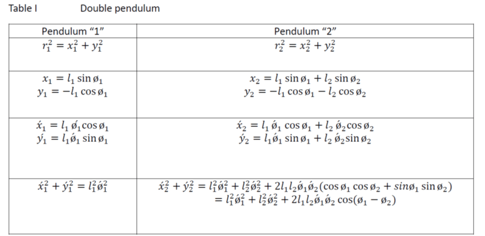
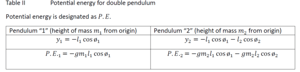
In Cartesian coordinates the Lagrangian expression for kinetic minus potential energy is

L = T – V = ½m₁(x’₁² + y’₁²) + ½m₂(x’₂² + y’₂²) – m₁𝑔y₁ – m₂𝑔y₂  .     (29)

Using the table as a guide, this expression may be transformed from Cartesian coordinates x₁, y₁, x₂, and y₂ to generalized coordinates ø₁ and ø₂, reducing the number of dependent variables by half.

L = ½(m₁ + m₂)𝑙₁²ø‘₁² + ½m₂𝑙₂²ø‘₂²+m₂𝑙₁𝑙₂ø‘₁ø‘₂ cos (ø₁ – ø₂) + (m₁ + m₂)𝑔𝑙₁ cos ø₁ + m₂𝑔𝑙₂ cos ø₂ (30)

Clearly, the complexity of this problem is greater than for the simple pendulum. If we make assumptions that m₁ = m₂ and 𝑙₁ = 𝑙₂, it becomes a little less complex.  Dividing both sides of the equation by the pendulum lengths, 𝑙, gives

L/𝑙 = m𝑙ø‘₁² + ½m𝑙ø‘₂² + m𝑙ø‘₁ø‘₂ cos (ø₁ – ø₂) + 2m𝑔 cos ø₁ + m𝑔 cos ø₁  .   (31)

Applying the Lagrangian differential expression (equation 2) for ø₁ gives

2m𝑙ø“₁ + m𝑙ø“₂ cos (ø₁ – ø₂) – m𝑙ø‘₂² sin (ø₁ – ø₂) + 2m𝑔 sin ø₁ = 0 .  (32)

Likewise, the Lagrangian differential expression for ø₂ is

m𝑙ø“₂ + m𝑙ø“₁ cos (ø₁ – ø₂) + m𝑙ø‘₁² sin (ø₁ – ø₂) + m𝑔sin ø₂ = 0.   (33)

This procedure has produced two intertwined (coupled) second order differential equations in the generalized coordinates ø₁ and ø₂ including their first- and second-time derivatives.  There exists no closed (simple algebraic) solution for these equations even though they fully specify the system’s motion. They may be solved numerically. 

How would one go about a numerical solution?  We need a starting position for ø₁ and ø₂ and starting angular velocities, ø‘₁  and ø‘₂.  As an example, begin with the initial angular velocities ø‘₁ and ø‘₂ = 0, and starting positions ø₁=𝜋/2, and ø₂ =𝜋.  Put these into the expressions (32), and (33); then solve for the unknowns ø“₁ and ø“₂ :

 ø“₁ ≅  Δø‘₁/Δt = – 𝑔/𝑙                  (34)

ø“₂ = 0                  (35)

After this first-time step, Δt, Δø‘₁ ≈ -𝑔Δt/𝑙, Δ(Δø₁) ≈ -𝑔Δt ²/𝑙 and ø‘₂ = 0; new approximate values for ø₁ and ø₂ may then be determined for the first time-step. Substituting these together with their derivatives allows the process to repeat for a second time-step: new values for ø“₁ and ø“₂ are then determined, and the process repeats for a third step, etc. There are finite-difference formulas for derivatives, which are very good, but not perfect, approximations (for example, the Runge-Kutta method).  As one quickly realizes, this becomes a problem suitable for computers. Typically, in a digital solution, one would test and then adjust the size of the time step so that the calculated movement is not coarse, and accuracy improved.  For each time step and with each new set of values for ø‘₁, ø‘₂, ø₁, and ø₂, equations (32) and (33) in their finite-difference approximations advance the motion forward for each successive new time interval. For a graphical illustration of the solution, one may consult MyPhysicsLab.com/pendulum/double-pendulum. https://www.myphysicslab.com/pendulum/double-pendulum-en.html

A Small angle approximation for double pendulum. To simplify the double pendulum problem, as was done in the previous example for the simple pendulum, one may specify that only small angles are allowed for ø₁ and ø₂. One then writes (in radians) a more tractable expression for the kinetic and potential energies using the approximation (in radians) ø ≈ sin ø ≈ x/𝑙.

Designate the horizontal deviations for each mass as x₁ and x₂.  The total kinetic energy for the two masses is

½m₁x’₁² + ½m₂x’₂²,        (36)

where x’₁ and x’₂ represent the horizontal velocities of the masses.  The potential energy for each pendulum mass may be approximated using equation (21).

V = 2m𝑔𝑙 sin²(ø/2) ≈ 2m𝑔𝑙ø²/4  ≈ m𝑔x²/2𝑙.   (37)

Cartesian coordinates are the generalized coordinates used here.  Apply expression (37) for potential energy to the double pendulum having weights m₁ and m₂.   Realize that for the upper pendulum, any deviation of x₁, must support both weights (m₁ + m₂).  This gives

V _tot = x₁²(m₁+ m₂)𝑔/2𝑙₁ + (x₂ – x₁)²m₂𝑔/2𝑙₂.                  (38)

To simplify further, set m₁ = m₂, and 𝑙₁ = 𝑙₂. Then

V _tot  = m𝑔x₁²/𝑙 + m𝑔(x₂² – 2x₁x₂ + x₁²)/2𝑙         (39)

𝜕V _tot  /𝜕x₁ = –m𝑔(-3x₁ + x₂)/𝑙                                   (40)

𝜕V _tot /𝜕x₂ = –m𝑔(x₁ – x₂)/𝑙                                          (41)

The Lagrangian differential expressions for two pendula of equal mass and equal lengths attached in tandem and deviating slightly from their vertical positions are

x”₁ – 𝑔(-3x₁ + x₂)/𝑙 = 0                 (42) 

 and

x”₂ – 𝑔(x₁ – x₂)/𝑙 = 0.      (43)

These are solvable analytically as coupled second order homogeneous linear differential equations with constant coefficients.   The system’s movement has two “characteristic” frequencies, 𝜈₁ and ν₂ and angular velocities, 𝜔₁, and 𝜔₂:

𝜔₁ = 𝜔₀ (2 + √2)^½ = 𝜔₀√3.414       (44)

𝜔₂ = 𝜔₀ (2 – √2)^½ = 𝜔₀√0.586  ,   (45)

With 𝜔₀ = √(𝑔/𝑙)

The movement solution takes the mathematical form ^{(footnote 9)}

x₁ = a cos 𝜔₁t +b cos 𝜔₂t       (46)

x₂ =  c cos 𝜔₁t + d cos 𝜔₂t      (47)

The four unknown constants a, b, c, and d  are determined using initial values for x₁, x₂, and their initial velocities, x’₁ and x’₂.  The movement would depend on the values determined for these constants.

4. Solid rod double pendulum

An even more complex double pendulum consists of two hinged identical solid rods of length l , each having mass m.  The Lagrangian expression (48), using a mixed set of Cartesian and radial coordinates:

L = T – V = ½m(x’₁² + y’₁²+ x’₂² +y’₂²) + ½I(ø‘₁²+ ø‘₂²) –m𝑔(y₁ + y₂) .  (48)

For this example, the rotational, or angular, movement of the solid rods must be included in the expression for the total kinetic energy. The required moment of inertia for each rod about its center of mass is I = m𝑙²/12  ^{(footnote 7)}.  The parameters x₁, y₁, x’₁,  and y’₁ represent the position and velocity of the center of mass of the first rod.  The second rod has these parameters designated with the subscript “2”.  The parameters ø‘₁² and ø‘₂² are the squares of the respective angular velocities of the two rods about their centers of mass. These are needed for calculating their rotational energies. 

Cartesian and radial coordinates appear in equation (48). The radial system, however, gives more compact answers and reduce the required number of parameters.  One may use Table III to replace the Cartesian coordinates of equation (48) with the radial equivalent.

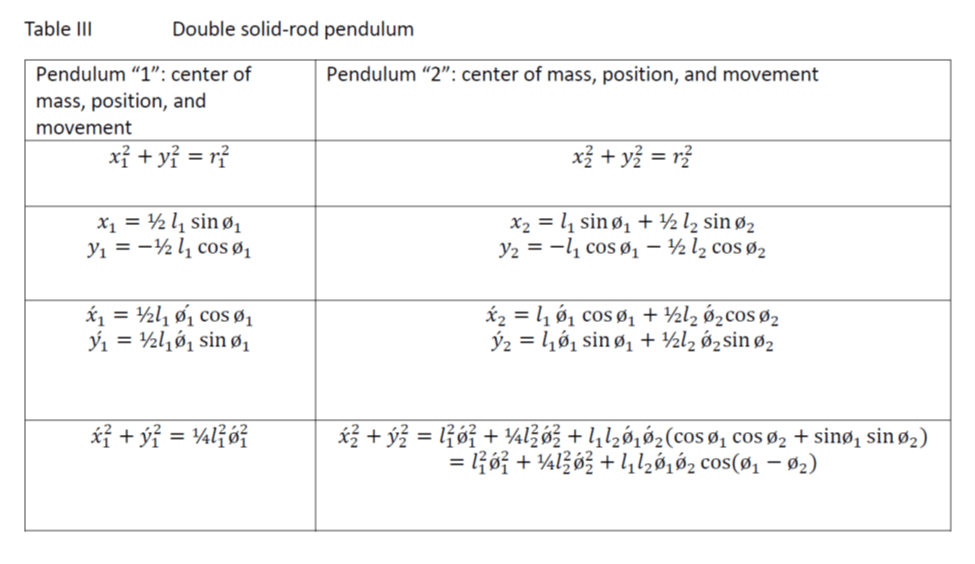
Table III is needed for the system’s translational kinetic energies, T.K.E  .   The rods’ rotational kinetic energies, R.K.E . are in table IV.  For 𝑙₁ = 𝑙₂ and m₁ = m₂, these results simplify to:

Substituting in equation (48) for translational (T.K.E ) and rotational (R.K.E.) kinetic energies, and using trigonometric identities yields

L/𝑙 = m𝑙[⅔ø’₁²+ ⅙ø‘₂² + ½ ø‘₁ø‘₂ cos (ø₁ – ø₂)] + m𝑔[1½ cosø₁ + ½ cos ø₂].   (49)

Compare this to the earlier equation (31) for the double pendulum with massless rods:

L/𝑙 = m𝑙[ø’₁² + ½ø‘₂² + ø‘₁ø‘₂ cos (ø₁ – ø₂)] + m𝑔[2cosø₁ +  cos ø₂].       (31)

Again, we have produced Lagragian equations of motion that are solvable only by numerical means.  Converting to canonical variables ø₁ and ø₂ has reduced the number of dependent variables by half.  The movements of the rods generally would not repeat.  (Perhaps, building a physical model with rods and well-lubricated hinges could be a more satisfying project for students rather than the tedious finite-difference procedures required for a numerical solution to equations (31) and (49).)

A small angle approximation for the example of the solid rod double pendulum would convert the differential equations of motion into homogeneous linear ones, which are solvable analytically.

Conclusion and links to modern physics

Historical figures that contributed to the least action Principle:

Lagrange

Euler

Hamilton

Jacobi

Quotations from Lanczos, and Goldstein concerning the least action principle.

 “Indeed, the idea of enlarging reality by including ‘tentative’ possibilities and then selecting one of these by the condition that it minimizes a certain quantity, seems to bring a purpose to the flow of natural events. This is in contradiction to the usual casual description of things. Yet we must not be surprised that for the more universal approach which was current in the 17^th and 18^th centuries, the two forms of thinking did not necessarily appear contradictory.  The keynote of that entire period was the seemingly pre-established harmony between ‘reason’ and ‘world’. The great discoveries of higher mathematics and their immediate application to nature imbued the philosophers of these days with an unbounded confidence in the fundamentally intellectual structure of the world” ^{(footnote 8)}.

 “…Classical mechanics remains an indispensable part of the physicist’s education. It has a twofold role in preparing the student for the study of modern physics. First, classical mechanics, in one or another of its advanced formulations, serves as the springboard for the various branches of modern physics.  Thus, the principle of lease action provides the transition to wave mechanics….  Secondly, classical mechanics affords the student an opportunity to master many of the mathematical techniques necessary for quantum mechanics while still working in terms of the familiar concepts of classical physics” ^{(footnote 5)}.

Analyzing problems of motion using the least action principle illustrates, among other things, that restraining forces, those unseen forces within solid structures and the forces at fixed points of attachments are not necessary for reaching a solution. Only the translational, rotational and the potential energies are required.  

For an orbiting planet’s movement around the sun, we need not include a planet’s rotation for a satisfactory solution. Nor must we include the movement of any internal molten magma for example, or any magnetic properties. Only the forces causing movement of the planet’s center of mass are required for an adequate description of the orbital path.  So, some forces, movements, and constraints may be ignored in these classical physics problems. However, accepting the possible existence of hidden movements, unseen constraints, or internal variables may have influenced views in the coming quantum mechanical era of physics.

Lagrange:  Lagrange’s name is attached to the method used in the previous examples.  Lagrange and his slightly older contemporary, Euler, are responsible for developing this method.  It goes without saying that the generalized coordinates of Euler need not be the orthogonal coordinates of Descartes. 

Hamilton: Hamilton’s method, considered to be a crowning achievement of 19^th century classical mechanics, was built on the procedures of Lagrange and Euler.  Hamilton used generalized momentum and position as the important variables (equation A4).  Jacobi, Hamilton’s contemporary, and a contributor to this method, coined the term canonical variables. Canonical variables of momentum and position and the Hamiltonian energy equation later found prominence in quantum mechanical theory, helping to establish modern physics in the first half of the twentieth century. 

Cornelius Lanczos ^{(footnote 8)}, in his textbook The Variational Principles of Mechanics, concludes that “the variational principles of mechanics continue to hold their ground in the description of all the phenomena of nature.”  This was a crowning achievement of nineteenth-century physics.

Appendix I: Summarizing the Lagrangian and Hamiltonian:

Lagrange:

The Lagrangian is the difference between kinetic and potential energies. 

T – V = L             (A1)

Hamilton:

The Hamiltonian may be given as the negative of the Lagrangian plus an action term.

-(T – V ) + Action = H (A2)

The student may wish to verify that

–L + Action = H = V – T + 2T = T + V   .              (A3)

Where the Action for each particle is p_i q’_i  or Action = q’_i  (dL/dq’_i ) when the particles’ potential is independent of velocity.  Total Action =⅀p_i q’_i (summed over all particles).

Represented in the familiar terms of velocity, v,  and position, x,

Action = ⅀m_i v_i ∙(dx_i/dt)    (A4)

Action as defined here has units of energy. The least action principle states that the paths of motion will be those for which the Lagrangian and the action are minimized… (the so called “laziness” of nature)^{(footnote 4)}. 

Appendix II: Suggested study questions:

1. Compare the least action principle with the Newtonian force method.

Answer: Going from Lagrange’s equation to Newton’s 2^nd Law is relatively easy. See footnote below.)  For the reverse procedure, the key is that the true and alternate paths must begin on the same point of the chosen generalized coordinates and all paths must also end on a single point. This sets the integration end points of the variation to be zero.

2. What are canonical variables.

Answer: These are designated p_i  and q_i  for generalized momentum and position and are used in the definitions of kinetic and potential energies.

3. Is orthogonality a requirement for canonical variables?

Answer: No

4. What can one say of the role given to time in classical mechanics of the 19^th century?

Possible answer to 4:   Because of the seemingly periodic nature of planetary movement and pendulum clocks, time seemed an understood concept in the nineteenth century: time should steadily and uniformly move forward.   In classical physics, time is typically described as an independent variable.  In the eighteen-hundreds, time seemed to be a “given” and somewhat boring parameter.  After Einstein, though, time acquired a more complex character.

5. What connections are there between the paired variables of energy-time (E  ⥋  t)  and momentum-distance  (p ⥋ x), which became important in quantum mechanics and relativity theory?

Possible answer to 5.   Relationships among force, momentum, distance, and energy may be a starting point for this comparison.

Energy = Force times the distance over which the force acts: dE = F∙dx     (A5)

and

Force = the rate of change of momentum:  F= dp/dt .    (A6)

Consider

dE dt = F ∙dx dt = (dp/dt) dx dt = dp ∙dx  .    (A7)

The pairing of energy with time and of momentum with distance feature prominently in physics, for example in quantum mechanics, Essay V https://ronaldabercrombie.blog/2023/12/15/v-a-conversation-about-quantum-mechanics/ and in general relativity, Essay VI https://ronaldabercrombie.blog/2023/12/17/vi-brief-outline-for-general-relativity/.

6. How may angular momentum enter the definition of action?

Possible answer to 6.  Action (as defined in equation A4) has units of energy. Another definition of Action is the energy product p_i ∙ q’_i  integrated over time; the resulting units of this are those of angular momentum.  Angular momentum may be expressed as energy multiplied by time or momentum multiplied by distance. (See pairing of ΔE  with dt  and 𝜕p with 𝜕x  in equation A7.)

Appendix III: Practice Exercises for High School Astronomy

This appendix was written primarily for high school science students and those without a specialized mathematical background.

A few concepts and equations, however, will be needed.  

(1) Force = mass x acceleration:                                                                  

(2) The gravitational centrifugal acceleration of an object in a circular orbit around a gravitational attraction center: Gravitational acceleration = (orbiting velocity)² / the radius of the orbit, r                  

(3) A second equation for gravitational acceleration: Gravitational acceleration = Universal constant of gravitation (G) x mass of gravitational attraction center (M)/(orbital radius)².                                                               

Combining equations (2) and (3) shows that the orbiting velocity of a satellite in a circular motion around the attraction center must be proportional to the square root of the mass of the attraction center divided by the orbiting radius:

(4) Orbiting velocity = √(G x M/ (orbiting radius)).

As the orbiting radius increases, the velocity of the orbiting satellite decreases.

Also, the satellite velocity decreases as the circumference of the orbit increases:

(5) The orbit period increases as Τ  =  2ϖ√((orbiting radius)³/G x M).

That the orbiting period increases with increasing orbiting radius to the power of 3/2 represents a special case of Kepler’s Third Law.

More energy is required to place a satellite into higher Earth orbit.  At the hypothetical orbit radius of infinity, the total energy is zero. In an actual orbit, the total energy will be less than zero, as the satellite is trapped by Earth’s gravity.  As it is pushed into a higher orbit by input of energy, the kinetic energy and the satellite velocity must decrease. Why? Because in a stable orbit the maximum kinetic plus potential energy is zero. When the kinetic energy exceeds gravity’s potential energy, it leaves Earth orbit as shown in the Fig. of the text on planetary movement.

Astronomical Observations of the Night Sky.

Once per month the shadow of the earth covers the moon, causing the monthly lunar eclipse.

On rare and irregular occasions and for those along a narrow path of Earth’s surface, a solar eclipse occurs, where the moon nearly exactly covers our view of the sun causing an astonishing, night-like, darkness in daytime.

To understand and appreciate these phenomena, we must know the distance of Earth to Sun and of the moon to the Earth.  Also, the radius of the moon and

Earth will be needed.

In meters these distances are given in the Table below.

	radius (meters)	Distance from earth (r) (meters)	Mass (Kgm)
Sun	6.96 x 108	151 x 109	~ 1.99 x 1030
Moon	1.74 x 106	384.4 x 106	~7.4 x 1022
Earth	6.36 x 106	0	~ 5.77 x 1024

Since the Earth and moon are approximately the same distance from the Sun, the Earth’s shadow on the moon is ~3.7 times greater in diameter than the moon’s shadow on Earth.  

The size of the moon’s shadow on earth during a solar eclipse is related to the size of moon, and its distance from Earth; the sun being much further away.

Radius of Earth compared to the radius of sun ~ 6.96/1.7 x 10² =  ~ 400. The distance from the earth to the sun compared to the distance from the moon to the Earth is  ~ 151 x 10⁹ /378 x 10⁶ =  ~ 400. This coincidence allows the earth’s shadow to cover the moon in the monthly cycles of lunar eclipse, which occurs ~ 13 times each year.

As an aside, the volume of sun compared the that of earth is (400)³ =  64 million.

For a solar or lunar eclipse, alignment of the Earth, moon and sun is required.

For a lunar eclipse the Earth takes the central position between sun and moon.

For a solar eclipse, the moon takes the central spot.

To visualize a solar eclipse, visualize a line through the center of the moon, Earth, and sun with an enclosing cone touching the surfaces of the sun and moon.  The tip of the moon’s shadow, the cone’s apex, points into Earth.

During a solar eclipse the moon’s shadow describes a circle of ~ 100 km radius on Earth’s surface.

For visualizing a lunar eclipse, the Earth takes the central spot. It may help to visualize a line through the center of the sun, moon, and Earth and a cone with its edge touching the sun and Earth’s surfaces pointing toward the moon. The apex of this cone goes beyond the moon. And the Earth’s shadow fully covers the moon during the lunar eclipse. This is because of the coincidence:  the Earth’s radius and Earth’s distance from the sun matches that of the moon and its distance from Earth, as described above.

As an exercise, use the table and equations to calculate the relative time periods, of a lunar month and an Earth year.

For calculating the time periods use equation (5) and the data shown in the table.

The ratio of the numbers calculated gives a value of 13.3 for the ratio of celestial lunar orbits (orbits using the fixed stars as a reference) to the Earth’s solar orbit.

Using the rotation of the earth and the distant sun as a reference, there are ~ 365.4 of Earth’s daily rotations as it returns in its solar orbit to an annual starting point. The moon circles the Earth every 27.3 Earth days. Using celestial time, this gives a ratio of 13.38, which shows a 0.08 discrepancy from the previous calculations.

Possible sources of discrepancy: 1.) The correct orbital radius should be used, that is, r should be the distance of the smaller body from the center of mass (M + m) of the two orbiting bodies, and 2.) The orbits are not circular but rather elliptical, which is another reason that the r used in the calculations may be incorrect.

What feature of the Earth’s polar axis causes the Earth’s seasons of summer and winter?

Answer:

The tilt of the Earth’ daily rotation relative to the plane of the earth’s path around the sun causes the northern and southern hemispheres to alternate in their semi-annual facing toward the warming sun. For the summer of each hemisphere, the sun’s rays are more concentrated on the Earth’s surface.

How does the density of the substance of Earth compare to that of the substance of the sun?

Use the volume of a sphere and the definition of density.  From the table,

Earth Mass is ~ 5.77 x 10²⁴  Kgm. Earth volume is 1.08 x 10²¹ meter³. Thus, the density of Earth is  ~ 5300 Kgm/ meter³.

By comparison, the sun’s Mass is ~ 1.99 x 10³⁰ Kgm. Sun’s volume is 1.412 x 10²⁷ meter³. Thus, it’s density is ~   1410 Kgm/meter³, less than the density of Earth. How can this be explained? Are the hydrogen atoms of the sun less densely packed than the atoms on Earth? No, but the atoms of which the Earth is composed have more massive nuclei than the hydrogen atoms that largely comprise the density of the sun.

Footnotes

¹The generalized coordinates need not be orthogonal coordinates.  They need only correctly describe a system’s energies.

²The Lagrangian expression, which uses energy, is equivalent to Newton’s Second Law, which uses force and acceleration.  Taking the expression for kinetic energy (as half the mass times velocity squared) and force (as the gradient of potential), Lagrange’s differential equation reproduces Newton’s Second Law.  In the simplest possible example, Lagrange’s equation (2) becomes mx” = – dV/dx = force .

³The adjusted Earth mass for this calculation:  m = m_Earth  M_sun /(m_Earth  + M_sun ) .

⁴ The time derivative of the Lagrangian and the action may be shown to be zero. This is related to the system energy being constant.  See Marion ^{6, p. 236}.

⁵ Herbert Goldstein, Classical Mechanics, Addison-Wesley, 1965

⁶ Jerry B. Marion, Classical Dynamics of particles and Systems, Academic Press, 1966

⁷ David Halliday and Robert Resnick, Physics, John Wiley & Sons, 1966

⁸ Cornelius Lanczos, The Variational Principles of Mechanics, Dover Publications, 1970

⁹ Shepley L. Ross, Differential Equations, Blaisdell Publishing Company, 1965