IV. Summary of Thermodynamics and Statistical Physics

 An Introduction to Some of the Basics

Thermodynamics is concerned with heat (thermos), movement (dynamics), and work; all are forms of energy. During the industrial revolution beginning in the 18^th century, engineers started examining heat as a source for movement and work … replacing draft animals, wind, and waterfalls. Classical thermodynamics began by pondering only visible movements.

Statistical physics, the intellectual companion of thermodynamics, includes the ubiquitous, random, and unseen microscopic movements associated with heat. A statistical approach to energy allowed more insights. As an example, the power of a steam piston was understood in the 1800s to result from many quadrillions (~10²³) of invisible molecules in a hot gas within the steam piston’s chamber. Maxwell and Boltzmann were among those to develop an understanding of microscopic molecular behavior, which provided energy for steam engines and locomotor trains and ushered forth the transportation and industrial eras.

Boltzmann (1844 – 1906)

Maxwell (1831 – 1879)

Chemical energy, like the heat energy of steam particles in a piston’s chamber, cannot be seen directly; chemical energy is contained in batteries and in the chemical bonds of fuel. Like heat energy, we see only the consequences of released chemical energy. American physicist, J. Willard Gibbs, helped provide an understanding of this in the 19^th century. Though there are other types of “unseen” energy that thermodynamics may consider, only heat and the energy contained within chemical bonds are included here.

Gibbs (1839 – 1903)

Thermodynamic work is visible.  In the 18th century, scientists and engineers began developing an understanding of how changes in temperature, heat, pressure, and volume could be harnessed for steam (or other) engines and locomotor propulsion.  They proceeded with the definition of work as force times the distance moved (d(Work) = F∙dx); it follows that the work of a piston may be expressed as the internal pressure within the piston’s cylinder multiplied by the change in the chamber volume as the piston is pushed forward.

                d(Work)=F·dx=(F/Area) · (Area·dx) = P·d(Vol)   (1)

Pressure, P , and volume, (Vol), then became preferred variables for the piston’s repeat cycles.  (Temperature and entropy, soon to be defined, may also be used.) The French physicist Sadi Carnot, in the 19^th century, showed how one could calculate the maximum work output theoretically possible in a “Carnot” cycle of an ideal engine by using pressure, volume, heat energy, and temperature as variables. In the Carnot cycle, two legs of the pressure-volume circuit occur at fixed temperatures; the other two legs occur at fixed amounts of heat energy within the piston’s chamber. For the constant temperature portions, heat must be added or removed reversibly as the work cycle progresses. For the constant energy (the adiabatic) portions of the cycle, temperatures fall (or rise) as heat is reversibly converted to (or extracted from) work.

Any ideal (reversable) pressure-volume loop may be imagined by combining smaller Carnot cycles: the adjacent internal legs of adjoining Carnot cycles cancel in forming an arbitrarily shaped work loop. As the loop repeats, some of this energy is captured as work; an ideal Carnot-cycle engine’s efficiency may be determined if the hot and cold operating temperatures are known.

Heat is a form of invisible thermodynamic energy. The heat energy that we cannot see but that we sense with detectors in our skin was difficult for scientists and engineers to precisely quantify early in the development of thermodynamics. This was because the temperature itself was hard to quantify. It was relatively easy to determine if one object had a higher temperature than another. However, a quantitative scale for temperature depended on the instrument one uses to measure it. For example, the expansion or contraction of a liquid such as mercury or alcohol in a traditional thermometer, the coiling or uncoiling of a metal spiral found in a garden thermometer, or the pressure increase of an ideal inert gas held at constant volume could be used to describe, define, and assign a scale for temperature. A thermometer based on the behavior of an ideal gas would eventually become the scientific standard.

The Celsius scale (°C) defines a range of temperatures of pure water from freezing to boiling: zero °C for freezing and 100°C for boiling (at sea level). There is no theoretical upper limit for temperature as there is no upper limit for heat energy, but there is a lower limit. At the lower limit, a minimum of microscopic particle movements defines negative ~273.15 °C as the base of the Celsius scale. The Kelvin scale (°K) assigns zero to this temperature. Kelvin temperature, named for Lord Kelvin (William Thompson, 1824-1907), is used in any scientific discussion of thermal energy.

Much earlier, Count Rumford (Benjamin Thompson, 1753-1814), while supervising the boring of cylinders for use as brass cannons by the Bavarian military, realized that the frictionally generated heat energy, and the work of boring these cannons were intrinsically related. This provided an early basis for formulating the first law of thermodynamics.

Heat and work represent two interchangeable energy forms, as James Joule stated explicitly in 1854 based on the careful measurements of this largely self-taught scientist. The First Law of Thermodynamics recognizes that the sum of heat and work energy is a fixed quantity for any thermally isolated, or adiabatic, system. When considering internal combustion engines, we recognize that chemical energy (in the form of gasoline, for example) may be converted to heat and, through the cylinder’s combustion pressure, into work. So, chemical energy in the fuel for our cars or in the battery energy that may propel them must be included when thinking about energy conservation and the potential for doing work.

Kelvin temperature is not equivalent to heat; however, these concepts are closely related.  This may be seen in the temperature and heat-content relationship defining entropy. Physicist Rudolf Clausius (1822-1888), in 1865, made the definition:

Entropy = S = (Heat content)/Temperature = Q/T  .   (2)

There are other ways to compare heat with temperature, but equation (2) provided a useful framework for much of the understanding of thermodynamic principles that were to follow. 

Microscopic molecular movements associated with heat, which were recognized in the 19th century, led to a statistical definition of entropy. In statistical mechanics, entropy is related to natural random movements (the disorder) ― of gas particles for example. The Second Law of Thermodynamics states that this disorder never spontaneously decreases; any system, say a collection of gas particles, will become more disordered as it progresses toward equilibrium. The maximum disorder at equilibrium defines the “ground state”, and any deviation from progression towards the ground state occurs only temporarily, in special or contrived circumstances, and limited space. The second law requires that the entropy enclosed within a fully isolated system must never decrease.

It will be helpful to begin this discussion of classical thermodynamics with a summary of terms. These will include four thermodynamic potential energy state functions.  The state functions (of Table II) were introduced as scientists began seeking ways of evaluating different circumstances under which some variables could be allowed to change while others were required to be held constant.

Work, heat, and chemical potential all represent types of energy; these are given quantitative expression using the parameters (variables) shown in Table I. There are different combinations of heat, work, and chemical energy for each of the thermodynamic energy state functions of Table II. There is a different set of natural variables for each state function (Table III); each state function has its usefulness for specific conditions, in which some parameters (in bold print of Table III) are held constant, while others (the natural variables) may change.

*System energy change defined for changes in entropy S, volume V, or mole content η (extensive variables) at constant temperature T , pressure P , and chemical potential, μ  (intensive variables). The equality in these expressions corresponds to reversible processes; irreversible processes must be represented by an inequality^{(note 2)}.  The variables not in bold print and appearing in infinitesimal form (such as dS, dV, and dη  in the first line of Table III, for example) are termed the natural variables, of which there is a distinct set for each of the listed four state function.

Infinitesimal changes in the system energy U (first line of Table III) may be divided into a work portion (-P· dV ), a chemical energy portion (μ·dη ), and a heat portion (dQ) as shown by dU=dQ – PdV + μdη ≤  TdS^{(note 1)} – PdV + μdη . The physics student will recognize that the negative sign for work (–PdV ) in these expressions signifies that this term represents work done by, rather than work done on, the system. Work, pressure, and volume were familiar concepts well before the 18^th century.

By the 19^th century, the concept of chemical energy was added to thermodynamics by the American physicist, J. Willard Gibbs (1839-1903). The Gibbs free energy of Table II includes amounts (mole content), 𝜂, of a chemical substance and a second factor given the title of chemical potential, 𝜇. Mole content is defined by a reactant’s (or reaction products’) molar amounts (extensive variables). Together with the chemical potential (an intensive variable), it quantifies the reaction energy.

The Gibbs chemical potential is defined as the released (or absorbed) chemical energy per mole at constant temperature and pressure.  This energy may be apportioned into parts; one portion ΔG₀ represents the energy difference at chemical equilibrium.  If the reaction has not yet reached equilibrium (or if occurring through an irreversible process) ^{(note 2)}, a deviation from ΔG₀ may be assigned an energy amount, ΔG₁.  The energy of a chemical reaction may always be expressed as ΔG₀ + ΔG₁ with ΔG₁ diminishing to zero for reversible processes and for the equilibrium condition.

The Gibbs energy appears in the definition of a reaction’s equilibrium dissociation constant, K_d.  The mathematical relationship for the example (A ⥊ B +C) being K_d = B ∙C/A = exp (-ΔG₀/kT ). The symbol A represents the equilibrium molar amount of the reactant.  B and C represent the equilibrium molar amounts of the dissociated products.  ΔG₀ is the Gibbs free energy difference at equilibrium between reactant and products. 

Temperature and pressure are the two natural variables for the Gibbs free energy of Table III.  One sees from the definition of the equilibrium dissociation constant that K_d would be greatly influenced by temperature but generally it is influenced less by changes in pressure. Gibbs energy is useful for predicting a reaction’s direction and its outcome. Once two sides of the reaction have reached chemical equilibrium at a designated temperature and pressure, ΔG₀ = –kT ln  K_d , and no further net conversion takes place^{(note 3)}.

Statistical physics. Much was accomplished using classical thermodynamics: it facilitated the understanding of steam engines and could be useful in solving other problems. However, statistical mechanics of the nineteenth century provided greater insights.

Entropy, heat, and temperature, one may argue, had been loosely defined in classical thermodynamics. Statistical physics provided more specifics. This required recognizing the inherent random microscopic molecular movement within all matter, an improved definition of temperature, and a concept termed the phase space. To illustrate entropy using phase space, textbooks often use the example of a mole of an ideal gas confined within a specified volume. Let this volume contain a total of ~6 x 10²³ (~one mole) of inert point molecules. Each molecule must have mass, three orthogonal components of velocity and three orthogonal components of position. (“Point masses” in an ideal gas are assumed to occupy insignificant space.)

So, there are ~36 x 10²³ coordinates required to describe a mole of gas in phase space: ~3 x 6 x 10²³ for location and ~3 x 6 x 10²³ for momentum. This being such an enormous number, physicists required other practical ways beyond classical mechanics to discuss entropy and heat energy.

A single point in phase space represents one particle. Each of the many points in six-dimensional phase space will change position and momentum as random interactions occur between particles and against the container walls. These point representations of particles, however, do not contact one another in the six-dimensional phase space: even during the physical collision of two particles, in which they would momentarily reside at the same three-dimensional location, they possess different momenta. Conversely, if two molecules have the same momenta, they have different locations. This holds true unless two particles become one, forming a chemical pair, which would never occur for an ideal gas of inert particles. So, in the imagined six-dimensional phase space, points representing molecules of an ideal gas never make contact. Also, in this six-dimensional phase space, the “density” of these points does not become uniform: particles having greater momenta will be located in less dense regions of the momentum portion of six-dimensional phase space.

Some basic simplifying statements about “point molecules” may be made.  If the temperature and volume of the confined gas are constant, the internal pressure and kinetic energy remain constant.  Summing in three dimensions over all the 6.02 x 10²³ particles of a mole of an ideal gas, the value

The total kinetic energy is fixed in this example, and the Boltzmann constant , k, and the Rydberg constant, R, are defined by expression (3). A calculation of

represents the average single-particle energy for one of three orthogonal directions of motion. All three orthogonal directions are equivalent for these gas molecules and the sum of the average values for momentum squared must remain constant; These average values form the surface of a “sphere”

in the three-dimensional momentum portion of six-dimensional phase space.

Phase space and entropy. Phase space may be used as the basis for a more complete and detailed definition of entropy.  Entropy, first defined by the ratio of heat to temperature, may be re-calculated for an ideal gas by using volume and temperature as variables. By taking the average momentum to replace temperature, the entropy for a fixed number, N₀, of ideal gas particles may be re-expressed in six-dimensional phase space using a conventional allowed volume and the average particle momentum as given in the following calculation.

Assuming the total internal energy to be constant (dU = 0) and a fixed number of particles (dn = 0), and using the differential expression from Table III gives

dU = dQ – PdV  = 0      or          (4)

dQ = PdV                            (5)

Clausius’ thermodynamic relationship, S =Q/T  with T constant requires that

dS=dQ/T  ^(note1)  .             (6)

Also, using the useful equation for a gas of ideal inert particles:

PV=nN₀ kT  .     (7)

After substituting for temperature and dQ  in these expressions (5), (6), and (7) and integrating the infinitesimal dS  using volume as the independent variable, we identify the change in entropy ΔS   per mole n resulting from the expansion of volume at constant temperature to be:

ΔS_V  = N₀ k ln(V_f/V_i) = k ln(Δw_V ^No ) = k ln(ΔW_V),           (8)

where the expression ΔW_V =  (Δw_V ^No ) = (V_f/V_i)^No  may be identified with the system randomness: the change in an individual particle’s randomness (at a constant temperature) is given by the ratio of its final to its initial allowed volume. It seems reasonable that if a particle is allowed to move through a space that is twice as large, then it possesses twice the randomness…twice the “freedom to roam”. The total system randomness is taken as the product of the randomness of each particle. This requires the exponent, N₀ in equation (8).  Total entropy is represented by the natural logarithm of the randomness product of all particles. Temperature was held constant for this calculation.

If volume is held constant instead and temperature is allowed to increase by adding heat, the change in entropy may be calculated using a similar procedure (Appendix) ^{(note 4)}:

ΔS_T = 3N₀  k ln (T_f/T_i)^½  .         (9)

The factor 3N₀ represents three orthogonal directions of movement for each of the N₀ particles within a mole of gas.

A combined expression for entropy when both temperature and volume are allowed as independent variables:

ΔS_T+ ΔS_V  = k ln(ΔW_T)+k ln(ΔW_V)=kN₀  ln (Δw_T ·Δw_V)=

3N₀ k ln [(T_f/T_i)^½·(Δx_f/Δx_i)].       (10)

The volume shown in equation (8) has been replaced with the cube of an allowed distance parameter, Δx, in equation (10). If one sums the entropy of each of the contributing spaces, the total entropy is represented by the log of the product of the phase space for each contributing part. Total phase space volume may be seen represented in equation (10) as ΔW = ( Δw_T ·Δw_V)^No.

One may now refine this relationship between entropy and the system’s randomness by changing from the variable of temperature to the variable of momentum. All parameters are not of equal utility in physics. Momentum is fundamental; temperature is not; classical temperature depends on the measuring devise. It is usually preferable for phase space to be re-expressed as a combination of the more fundamental parameters of momentum and position in an expression similar to the one below (11).

ΔW = ΔW_p · ΔW_V = (Δw_p· Δw_V)^No        (11)

One concentrates on the momentum portion, w_p^No or W_p . How is temperature in equation (10) to be replaced with a parameter for momentum in equation (11)?

At constant volume, the ideal gas temperature is only related to gas pressure as PV = NkT .  Gas pressure is directly related to the instantaneous forces of all particles striking the walls of their container. These forces result from changes in the momentum of many individual particles (each imparting an impulse to the container walls); the totality of these impulses is collectively and uniformly distributed over the container walls. Thus, temperature (which is related to pressure at constant volume) would also be related to the collective forces of all these particles’ momenta or the collective particle’s average momenta. This may be seen directly in the expression shown in equations (3).   The average of the particle momentum square in one (j) direction must be proportional to temperature in accordance with the relationship between temperature and average squared momentum:

Each particle, moving in accordance with its kinetic energy and its individual component of the total momentum, contributes a small part to the total pressure. As the total momentum “volume” of phase-space is represented by the product of the individual particles’ momenta, one might (erroneously) predict the phase-space temperature to be related to the product of the square root of each individual particle’s “temperature.” However, the average of the squares does not equal the square of the averages. Also, temperature may only be defined as an average value for a collection of gas particles, not as an individual particle value. Nevertheless, using the reasonable assumption that an “average temperature” for each individual particle over a long time is equivalent to the average temperature of all particles taken at one point in time (similar to J. W. Gibb’s rule), one is allowed the conceptual leap from temperature to the average particle squared momentum as represented in these equations. The average energy of an individual particle

is related to the common value for temperature.

Heat capacity.  The change in heat content of an object (ΔQ ) may be defined in classical thermodynamics using the change in temperature multiplied by a heat capacity as (ΔQ = heat capacity· ΔT ).  The heat capacity of a gas must specify either a constant volume or a constant pressure, C_V or C_P, as described in a footnote ^{(note 5)}.

The capacity of any material to accommodate heat may also be influenced by changes of state from solid to liquid or from liquid to gas as heat is involved in these transitions. Heat capacity of a realistic gas would be influenced by an array of molecular properties including the ability of realistic gas particles to vibrate and freely rotate. So real gas molecules are more complicated.

The specific heat capacity of an ideal gas of point particles at constant pressure is shown in Appendix ^{(note 4)} as  C_P = C_V  + N₀ k = (2½) N₀ k . The heat capacity of an ideal gas at constant volume is C_V  = (3/2) N₀k  . These relationships illustrates that if the volume is allowed to increase at a constant pressure, an ideal gas accommodates more heat by the amount N₀k.

One cannot escape noticing a relationship between heat capacity at constant volume and entropy change at constant volume. If temperature is used (in place of momentum), then the entropy change at constant volume may be expressed as

ΔS_T = (3/2) N₀ k ln(T_f/T_i )= C_V  ln(T_f/T_i ) .      (12)

Summary: the entropy of equation (10) is related to the randomness of the system, which may be defined using an accessible volume in a six-dimensional phase space. Temperature is easy to measure with a thermometer for a collection of particles. It remains vague for a single particle: only an average temperature of a single particle would make any sense. Whereas the momentum of each particle is specific, it would be difficult to measure. We calculate the average momentum of a particle by taking the temperature of a collection of particles. Momentum, being fundamental in physics, is generally considered better suited for the phase space representation.

Quantum mechanics incorporates an inescapable granularity of nature when examined in small spaces. The factor (Δ x) imbedded within equation (10) would identify an allowed accessible element of space.  If used in the context of quantum mechanics, there must be a minimum for an allowed distance times an allowed momentum according to the Heisenberg uncertainty principle (Essay V https://wordpress.com/post/ronaldabercrombie.blog/189).

This uncertainty principle states that a limit for the precision of the product momentum · distance (or for energy · time) must be represented as

Δp·Δx ≥ ħ/2    ,                 (13a)

or

(ΔE·Δt ≥ ħ/2)   .               (13b)

See answer to Question 5 in Appendix II of https://ronaldabercrombie.blog/2023/12/12/iii-the-least-action-principle-of-classical-mechanics/

Though classical phase space requires continuous and precise values, the uncertainty principle within small, confined spaces in quantum mechanics makes such a minute precision impossible.  The reciprocal relationships and the quantum mechanical granularity and uncertainty in small spaces is discussed briefly in Essay, V.

Now, return to a elementary statistical description of gas particles, for which quantum mechanics is not required.

As a useful exercise consider Maxwell’s velocity distribution.    Equation (16) may be derived from standard kinetic theory for a system of randomly moving gas particles.  In a three-dimensional momentum space, a random or Gaussian normal probability distribution of the momentum, p, of gas particles is represented as

The function 𝛷(p) represents the partitioning of particles of an ideal gas using their momenta (or kinetic energies) as the important variable. To calculate the average kinetic energy for one orthogonal direction, [p_i²]_ave /2m, Maxwell used the relationship of equation (14) .  

This Cambridge-trained mathematician knew:

Taking equation (14) for the partition function 𝛷(p) and normalizing using equation (15), gives 

and together with p² = p_x² + p_y² + p_z², this yields

Each particle of a gas has its individual momentum.  A single particle’s average kinetic energy (the average energy for the full spectrum of allowed values of momentum) is

confirming the value of ½ kT  for the average kinetic energy for each of the three orthogonal directions of a point particle’s motion (equation 3) for an ideal gas and confirming a random distribution of momenta for particles of an ideal gas.  This gas particle energy distribution is attributed to Maxwell^{(note 1)}.

The partition function of statistical mechanics and the phase-space concept provided scientists in the 19th century with methods for dividing the exceptionally large number of particles into manageable sub-compartments. The partition function uses energy for this task. Phase space uses compartments based on position and momentum.

Counting in Statistical Thermodynamics

1. The Maxwell-Boltzmann partition function: Maxwell’s insight regarding the energy distribution and partitioning of distinguishable molecules within a gas (and Boltzmann’s similar reasoning applicable for any classical energy distribution) can be expressed using  d{ln(n)} = dn/n and

so,

d ln(n_j ) = –β(Ԑ_j);  or n_j = Const · exp(-β Ԑ_j )                       (19)

with β =1/kT  . The average number of particles with kinetic energy equal to Ԑ_j may be represented as

whereas

represents the count of particles of all energies. The negative sign at the far right of equation (18) is a reminder that, on average, fewer particles will be found in higher energy categories. The average number of entities in a sub-grouping may be expressed using equation (19) or using momentum as in equations (14) and (17).  Boltzmann put forward the general relationship of equation (20), where Ԑ_i represents an energy level of a system. Equation (20) shows the average population of the i^th  energy level.  For Maxwell-Boltzmann particles,

The inclusion of the energy reference term Ԑ_MB allows the inclusion of a defined energy-zero, i.e., an energy base. This would be at the temperature of absolute zero for the imagined ideal gas described by Maxwell.

Distinguishable and indistinguishable particle counting. Equation (20) represents energy partitioning for distinguishable particles. Why must one stipulate that the atoms or molecules of an ideal gas should be considered as distinguishable one from another… even though they may appear on superficial inspection to be identical? A way to ask this question is to ask if one molecule or atom within such a collection could be set apart from all the others. For atoms or molecules, this distinction may be accomplished, with a subatomic, or nuclear isotope for example. Therefore, molecules within an ideal gas are distinguishable. They may be tagged and set apart from one another. A further description of (20) is found in the footnotes^{(note 6)}.

The quantum mechanical statistical descriptions of Bosons or Fermions, which are indistinguishable particles, require Bose-Einstein or Fermi-Dirac partition functions.

2. The Bose-Einstein Partition Function. Bose-Einstein particles are indistinguishable entities, meaning that labels or identification are not possible. A notable characteristic of Bose-Einstein particles is that any number can occupy a single energy state. The expression for the energy partitioning function of Bose-Einstein particles representing the average probability of finding these entities within a given energy level Ԑ_i, is

Incorporating Ԑ_BE provides a foundational energy base. Photons are indistinguishable Bose-Einstein particles. Interested students may verify that Equation (21) aligns with Planck’s formula for energy distribution within a “black body” cavity containing a “gas” of photons (Essay V). Additional details on Equation (21) are provided in the footnotes ^{(note 6)}.

3. The Fermi-Dirac Distribution applies to electrons and protons, which like photons, are indistinguishable, one from another. However, electron populations allow only two per quantum state. Each electron within an atomic orbital state possesses a magnetic property termed spin. Only one electron with spin “up” and one with spin “down” is permitted per atomic orbital. This differs from Bose-Einstein entities, which allow unlimited numbers within states. The Fermi-Dirac distribution is the quantum mechanical basis of the two-electron requirement for forming chemical bonds and adheres to the Pauli exclusion principle for Fermions (See Essay V). The statistical distribution function for fermion-type particles is

The reference energy is designated as Ԑ_FD.  Another description of equation (22) is given in the footnotes ^{(note 6)}.

Overview of Entropy and the Universe. An essential thermodynamic conclusion perhaps warrants repetition: the inevitable progression towards maximal disorder. The freely moving molecules of a gas—or all matter within the universe—progress towards a state of “maximal disorder.” According to thermodynamic principles, this progression is universal and unavoidable, though temporary local exceptions may occur. A notable exception is life on Earth. Life represents a temporary steady state amidst the progression to disorder. Nonetheless, the equilibrium state that ultimately prevails and to which all matter inevitably progresses, is one of maximal disorder according to the second law of thermodynamics.

Biological cells, the foundation of life on Earth, contain a limiting membrane that maintains order within its enclosure. However, in the broader context of the universe, such occurrences are rare. Life on Earth creates the mistaken impression of abundant order. Yet, this beautiful, ordered, entropy-defying steady state constitutes a very small part of the universe, at least that is the conclusion based on current observations. https://ronaldabercrombie.blog/2024/05/14/where-physics-and-biology-intersect/

Appendices

Problems (Some questions and possible answers)

Consider the changes that must be made if an MB gas is not ideal. For example, allow:

particle-particle interactions, particles having a finite size, or particles having rotational or vibrational energies.

Answer: One method for compensating for the finite size of gas molecules is to subtract this space from the volume of the gas. If there are Van der Waals type particle-particle interactions, these must also be included as a source of deviation from the ideal gas equations. Van der Waals forces are electrostatic in nature. They result from induced dipole-dipole interactions and extend beyond the touching surfaces of the gas particles. If gas molecules have structure, then they may have linear vibrations. Such vibrations represent an energy component for the system. Molecules with structure may also rotate.  One expects the energy to increase by an amount kT/2 for each gas molecule as vibration or rotation becomes a component of its energy.

Consider how the uncertainty of quantum mechanics changes the phase space formulation:   Uncertainty must be considered in a discussion of thermodynamics if quantum mechanical granularity and the lack of precision of momentum and position are important.  The Heisenberg relationship as described in Essay V would need to be included https://ronaldabercrombie.blog/2023/12/15/v-a-conversation-about-quantum-mechanics/.

Questions concerning the Carnot cycle:  Determine the efficiency of an ideal Carnot cycle engine in terms of the maximum and minimum cycle temperatures. What factors make an engine less efficient than an ideal Carnot engine?

Compare the physics of the Carnot Cycle, the Diesel Cycle, Jet engines (Brayton cycle), and refrigeration devices:

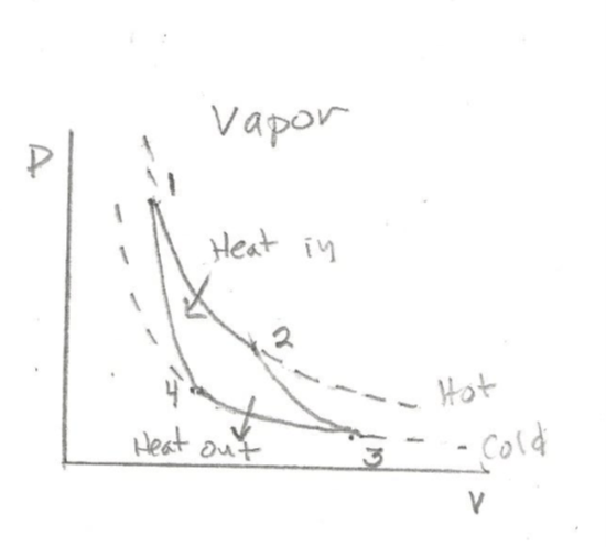
Answer: Steam engines, part of the industrial revolution, are external combustion engines using fuel, which is burned outside the work cylinder to generate steam heat. Heat is transferred to the work cylinder where steam is converted to power.

The ideal Carnot cycle (of external combustion steam engines) has four phases, two occur at constant temperature (1-2 and 3-4) and two adiabatic phases occur at constant internal heat (2-3 and 4-1)

P-V Diagram for Carnot Cycle

Internal combustion engines burn fuel inside the work cylinder. There are two types of these engines: gasoline, which are compact and use a spark for ignition, and Diesel, which require no spark, are larger, operate under higher pressure, and may use a variety of less volatile fuels. Diesel engines ignite fuel with highly compressed air which becomes sufficiently hot to automatically combust the fuel.

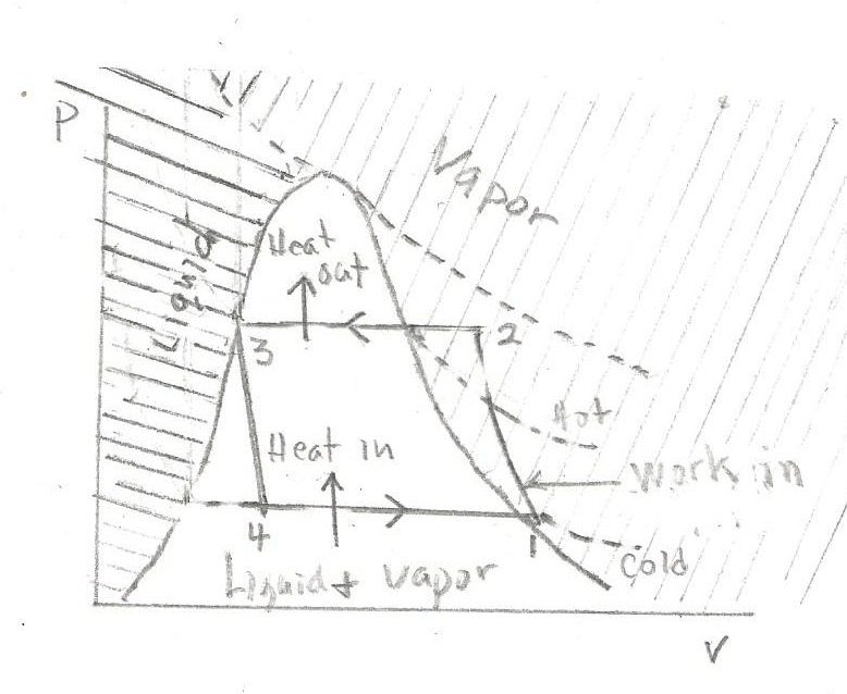
Figures are adapted from Thermodynamics by Çengel and Boles, Third edition, McGraw-Hill, 1997, and Morse, Thermal Physics, W. A. Benjamin, 1964.

“Heat in” in these figures signifies caloric energy, Q, put into the system, “Heat out” signifies caloric energy leaving the cylinder chamber.  The isotherms in the figures are shown as dotted lines

Diesel Engines

The Diesel cycle’s behavior can be explained using a P-V-T diagram, similar to the Carnot Cycle in thermodynamics. The ideal Diesel cycle includes four steps. In step 1-2, air is compressed to a high temperature that ignites the fuel. This step is isentropic, meaning entropy, Q/T, not the heat energy) remains constant. The diagram shows the temperature via dotted-line isotherms.  Stage 1-2 requires that work is put into the system as the piston is driven forward within the air-filled cylinder chamber. Following this, in stage 2-3, fuel is injected, ignited by the high temperature and pressure, and the piston stroke commences, initially occurring under constant pressure conditions. Stage 3-4: during the second isentropic step of the cycle, work continues until the piston reaches the mechanical limit at the maximum volume of the chamber. Temperature is dissipated and the pressure drops during this step. Stage 4-1: Temperature further decreases as heated gas exits the piston chamber, with no additional work occurring as the piston remains stationary. The cycle then begins anew.

P-V Diagram for Diesel Engines

P-V Diagram for Jet engines (Brayton cycle)

The thermodynamic process of jet engines is similar in many respects to Diesel engines. Step 1-2 is an isentropic compression. Step 2-3 involves constant pressure heat addition by fuel combustion. In step 2-3, as in Diesel engines, compression ignites the jet engine fuel. Step 3-4 is an isentropic gas expansion within the turbine. Step 4-1 involves heat and gas rejection at constant pressure. This step is unlike that of the Diesel engine as it occurs at constant pressure.

Refrigeration devices

Refrigeration devices use a similar pressure, volume, and temperature diagram as for Diesel engines, with some key differences:

• The refrigeration substance (refrigerant) changes phases between liquid and vapor and the refrigerant is not consumed contrasting with the fuel’s consumption in Diesel engines.
• The P-V cycle works in reverse compared to Diesel engines.
• Energy is supplied not by the Diesel fuel but rather by an external motor.

Notably, Rudolf Diesel managed a refrigeration company during his early career. Key parts of the system include an expansion valve and mechanical compressor. Various materials may be used for the refrigerant substance.

The refrigerant in these devices is found in both gas and liquid form and is contained within a sealed system. The system contains compressor and condenser sections. The ideal refrigeration cycle includes four steps:

1-2: The gas/liquid undergoes compression, resulting in increased temperature and pressure.

2-3: As the compressed gas/liquid increases the temperature, heat is lost from the system because of the cooler ambient temperature. During this phase, the refrigerant exists both gas and liquid phases under a constant pressure.

3-4: The pressurized liquid/gas refrigerant moves through the expansion/throttling valve, emerging as a cooler gas at lower pressure on the other side.

4-1: Post-throttling valve, the refrigerant at constant pressure absorbs heat from the environment as the gas volume expands. The pipes in this part of the system feel cold to the touch.

P-V Diagram for Refrigeration Devices

Footnotes (including additional problems)

^note1 For Heat energy and the pressure of an ideal gas,  accurate “bookkeeping” will be required.  The components of force on a container wall result from the movement of individual gas particles. For one of three orthogonal directions of movement,  force_x = (rate of change of momentum)_x.  Consider a volume V  in which N  particles reside; focus attention on a microscopic volume element, (dx)³, containing particles capable of striking the container wall surface (dx)² within a designated time. The time required for a particle, i , with velocity component, v_x,i, to transverse a length dx  in a direction toward the wall, imparting its impulse is given by dx/v_x,i.  The collection of particles within the container striking the walls produce an average continuous force (momentum change per second); this force, divided by area, A, and summed for all particles, ΔN , striking the wall within an elapsed time, dx/v_x,i, produces a pressure, P .  The pressure for one direction must be the same as the pressure for all directions as the gas system is isotopic.  Incorporating these factors leads to equation (A1), which may be expressed using a term for the average kinetic energy of a particle and/or the kinetic energy for the entire gas, U .

[Energy divided by volume has units of pressure. The factor ½ before the summation symbol signifies that half of the particles near the surface of the container move towards the wall and half move away. The doubling factor  within the first parenthesis must be included as the impulse results from the reversal of each particle’s momentum. These cancel one another producing the sum shown in equation (A1 and A2). The kinetic energy of each particle associated with one of the three orthogonal direction of movement is K.E._x = ½mv_x² . When the total average kinetic energy for all three directions is included in the expression (A1) a factor ⅓ is required. The tabulated density of gas particles in this calculation ΔN/Adx  must equal N/V  as this average gas density in the container must be the same everywhere.] The pressure, P , may be also expressed using the average density of the gas, where density is

and pressure is

Or equation (A1) may be re-arranged as

PV (=nRT) = ⅔U           (A3)

[A monatomic gas molecule would have three degrees of freedom; more complex particles possess additional degrees of freedom, for example, rotational and/or vibrational.]

^note2 In a fully reversible process, a complete pressure-volume loop would return the entropy to its initial value.  This applies for any of the state functions (U, G, F, or H), as they must not depend on the paths taken to reach the destination.  For a closed path, the thermodynamic extensive variable entropy, S ,

∮ d[S]_reversible = ∮ d[Q/T]_reversible = 0 .

Irreversible or dissipative processes are far more common. For these, the integral path shown above would underestimate the change in entropy and instead:

∮ d[S]_irreversible = ∮d[Q/T]_irreversible  > 0 .

As examples, the expansion of a gas into an opened vacuum, a realistic steam engine, a refrigeration device, or any processes involving friction would increase the entropy irreversibly.

^note3 Problems concerning energy released by a chemical reaction: These problems typically make use of the Gibbs energy, G ,which assumes temperature and pressure as natural variables or, alternatively, the Enthalpic energy, H , which assumes entropy (disorder) and pressure as natural variables.

For constant temperature and pressure, the equation for the equilibrium dissociation constant of a simple reaction is expressed as

K_d = B ∙C/A = exp (-[G₂ –G₁]/kT).  (A4)

As an example, take the formation of water from hydrogen and oxygen.

2H₂ + O₂ ⥊ 2H₂O .         

We know that this reaction is strongly favored to proceed to the right as water is a chemically stable molecule. Introducing the association constant K_a  (rather than the dissociation constant K_d)  one has

K_a = 1/K_d = exp([G₂ – G₁]/kT) ,               (A5)

This calculation must consider the energy required to break the O₂ and H₂ diatomic bonds to form atomic hydrogen and oxygen and the energy regained by these atoms as they combine to form water.

The Gibbs energy for many reactions may be found in reference books.

[For some problems, the Enthalpy, ΔH  or the Helmholtz free energy, ΔF , may be more useful than the Gibbs energy, ΔG .  For example, when temperature and volume are the natural variables: dF  ≤ –SdT –PdV + 𝜇d𝜂. For other purposes the Enthalpy, dH  ≤ TdS + VdP + 𝜇d𝜂, is useful, for occasions when entropy and pressure are required to be the natural variables.]

Suggestion: use the Gibbs free energy of a chemical reaction to calculate the equilibrium dissociation constant.

And use the measured energy released in an exothermic reaction under appropriate conditions and calculate Helmholtz energy.

^note4 Derive the formula relating entropy and temperature at constant volume

At constant volume, dQ = dU = TdS  or dS = dU/T  = 1½(nkN₀ dT )/T .    

(U = 1½NRT = 1½nN₀kT  as T is the only variable) .  After substitution and integration,

S_f – S_i = ΔS_T = 3nkN₀ ln [(T_f /T_i)^½] .        (A6)

note⁵ To determine the heat capacity of an ideal monatomic gas at constant pressure, begin with the expression of energy conservation (the first law of thermodynamics). From Table III, –PV in the expression of total energy represents work done by the system; From the first line of Table III,

dQ = dU + PdV    .           (A7)

Temperature (T) and volume (V) are the independent variables. Pressure is constant in this example, and one assumes one mole of gas (n=1). Define the heat capacity at constant pressure, C_P  as  [∂Q/∂T]_P .  

The partial derivative of the heat with respect to temperature at a constant volume is the heat capacity of the gas at constant volume. From equation (A7),  C_V= [∂Q/∂T ]_V = [∂U/∂T ]_V .

Heat capacity of the gas at constant pressure may also be extracted from (A7) using the total derivative:

dQ =[∂U/∂T]_V dT  + [∂U/∂V]_T dV + PdV

C_P = [∂Q/∂T ]_P =C_V ·[∂T/∂T ]_P + [∂V/∂T ]_P · [∂U/∂V ]_T  +P [∂V/∂T]_P   or

C_P = C_V  + [∂V/∂T ]_P · [∂U/∂V ]_T +P [∂V/∂T]_P .   (A8)

However, [∂V/∂T ]_P · [∂U/∂V ]_T   = 0 , as [∂V/∂T ]_P  = NR/const  and [∂U/∂V ]_T  = 3/2[∂kT/∂V] _T =0 .  Equation (A8) becomes

C_P = C_V + P ∙(𝜕V/𝜕T ) = C_V + P ∙(R/P) = C_V   + R .          (A9)

From (A7) and using the heat capacity of an ideal gas at constant volume, C_V = [𝜕U/𝜕T ]_V  = 1½R. 

The heat capacity of an ideal gas at constant pressure is

C_P = 2½R   (A10).

^note6 More on BE, MB, and FD statistics:

BE.  For Bosons, the total energy phase space of the collection of particles, designated as W , may be represented in (A11) using equation (19) as a guide.

The summation over the parameter r  includes all allowed values for boson numbers n_i  in each energy level, Ɛ_i .

Because there is no limitation for occupancy of Ɛ₁ , Ɛ₂, Ɛ₃, Ɛ₄, … etc., the expression for the BE partition function (equation A11) may be re-written as a summation over the occupation of each energy level.

Each of the sums in the product is represented by a similar mathematical expression (w_j for each energy level Ɛ_j).  Using the result of the infinite series,

Equation (A12) becomes,

As the log of a product is also the sum of the log of the individual terms, and because moving from denominator to numerator changes the sign of the log,

“Pulling out” a single sub-state, microstate, or energy level of interest i  by differentiation of (A15) by Ɛ_i and using the mathematical relationship, dW/W= d{ln(W)}, the expected occupancy number for the chosen level i  becomes, 

MB:  Maxwell-Boltzmann statistics are used to determine the average number of distinguishable particles expected to reside at a given energy level. The full collection of particle energy states including every allowed configuration may be counted using the index r .  Energy configurations are sub-divided into sub-states, identified as w_i ; each sub-state represents only a part of the full phase space, which is identified W. (Sub-states are typically numbered using the index, i, and by the lower case w.) The w_i  substates designate particles of each energy level as an “energy microstate”. 

Equation (A18) represents a grouping of energy states: n_i is the expected particle count having energy microstate level i as found in w_i ; N  is the full count of all particles in W .

Using this expression and equations (19) and (A11) as a guide for summing the full energy space,

Equation (A19) includes all possible energy states and all allowed combinations of occupancy numbers n_i and energy levels Ɛ_ithat are compatible with a fixed total number of distinguishable particles and fixed total energy. 

For Maxwell-Boltzmann particles, the distribution takes a comparatively simple form: The probability P (w_i) of each microsystem for each energy sub-state Ɛ_i in a Maxwell-Boltzmann distribution is represented as

the symbol A being the normalizing factor. MB particles are distinguishable; however, within a single energy level, these particles are interchangeable.  Every energy sub-level, a designated microstate, would be governed by an identical expression given in (A20). 

Summarizing, the average number of particles to be found in each energy sub-level may be expressed as

with the total

or

with  𝛽 = 1/kT  . 

A useful way of expressing equations (A21) is to mathematically “pull out” the average occupancy number for the energy level of interest by taking the derivative of W  in equation (A19) with respect to Ɛ_i . One may verify that this gives the result of equations (A21) as

FD: Fermi-Dirac statistics limit the number of indistinguishable fermion particles assigned to each quantum state.  This rule applies to electrons filling orbitals within an atom.  For each quantum mechanical orbital, only two electrons are permitted, one for each of the allowed electron spin states.  One designates that each identifiable energy state, r , may either be not occupied (n = 0 )  or occupied (n = 1).  Then

Here the expression

represents an energy microstate, Ɛ_r, of the collection of fermions. 

Changing the counting index from r  to i , the average occupancy number for energy level i , may be determined by differentiating W  (A23) by Ɛ_i to “pull out” the energy level of interest.

The result is

The number of particles N  in the system must satisfy.

The probability for occupancy of each energy level i may be expressed as

Using Ɛ_FD as the zero-energy reference for the Fermi Dirac particles.

[Spin state is just one of the quantum numbers identifying an electron confined within atoms. According to the Pauli Exclusion Principle, each electron must reside in a different designated quantum state. For two electrons within a single orbital space, their spins (and their magnetic moments) must be different. This becomes apparent when atomic electron energy levels are split by an imposed magnetic field.]

Useful references

Thermal Physics, Philip Morse, W.A. Benjamin, INC, New York, 1964

Elementary Statistical Physics, C. Kittel, John Wiley & Sons, fifth printing, 1967